CBDC and business cycle dynamics in a New Monetarist New Keynesian model

CBDC and business cycle dynamics in a New Monetarist New Keynesian model

Annukka Ristiniemi

Disclaimer: This paper should not be reported as representing the views of the European Central Bank (ECB). The views expressed are those of the authors and do not necessarily reflect those of the ECB.

Abstract

To study implications of an interest-bearing CBDC on the economy, we integrate a New Monetarist-type decentralised market that explicitly accounts for the means-of-exchange function of bank deposits and CBDC into a New Keynesian model with financial frictions. The central bank influences the store-of-value function of money through a conventional Taylor rule while it affects the means-of-exchange function of money through CBDC operations. Peak responses to monetary policy shocks remain similar in the presence of an interest-bearing CBDC, implying that monetary transmission is not impaired. At the same time however, the provision of CBDC helps smooth responses to macroeconomic shocks. By supplying CBDC, the central bank contributes to stabilising the liquidity premium, thereby affecting bank funding conditions and the opportunity costs of money, which dampens and smoothes the reaction of investment and consumption to macroeconomic shocks.

Keywords: Central bank digital currency, monetary policy, DSGE, search and matching.

JEL Classification: E58, E41, E42, E51, E52.

Non-technical summary

In the past few years, an increasing number of central banks have started to consider the potential provision of central bank digital currency (CBDC) to the wider public for payment purposes (Kosse and Mattei, 2022; Boar and Wehrli, 2021). Such a provision would raise several important policy questions, in particular for monetary policy transmission and financial stability, especially if CBDC were to replace bank deposits on a larger scale.

We investigate how the potential existence of an interest-bearing CBDC would alter the economy’s dynamics in response to a number of macroeconomic shocks. A key feature of a CBDC is its means-of-payment function (e.g. see Group of Central Banks 2020 or Panetta 2021 for the digital euro), which we emphasise by modelling the micro-foundations of a CBDC as a means of payment explicitly. To this end, we integrate a decentralised market in the spirit of Lagos and Wright (2005) into a New Keynesian dynamic stochastic general equilibrium (DSGE) model with financial frictions that is based on Gertler and Karadi (2011) by following the approach of Aruoba and Schorfheide (2011). In our model setup, CBDC and deposits are perfect substitutes and essential to pay for consumption. By combining the New Monetarist decentralised transactions with the New Keynesian business cycle dynamics, this approach is well suited to analyse the properties of deposits and CBDC as means of payment while at the same time it allows us to investigate the interactions of business cycle fluctuations, financial frictions and monetary policy with the payment functions of different forms of money.

In our model, an interest-bearing CBDC can be used by the central bank to separately influence the store-of-value and the means of exchange function of money. The central bank can thereby stabilise the liquidity premium, which is defined as the spread between the interest rate on CBDC and bank deposits relative to the return on government bonds, resulting in an additional channel through which monetary policy transmits to the economy.

Generally, we find that the presence of a CBDC does not significantly alter the properties of the model’s responses to the usual macroeconomic shocks and tends to dampen and smooth their transmission to core variables such as output and inflation. Regarding shocks to the liquidity premium, the existence of a CBDC stabilises the responses of output and inflation if such shocks affect money supply but amplifies them if money demand is impacted.

Importantly, monetary policy remains similarly effective in the presence of a CBDC. An increase in CBDC supply, which leads to a decrease in the liquidity premium, raises consumption, output, and inflation. The dynamic impact of CBDC on the economy is determined by how much the central bank adjusts CBDC supply to changes in the liquidity premium. The less the central bank reacts to the liquidity premium, the more the responses of output and inflation to macroeconomic shocks resemble those in the model version without a CBDC. Moreover, we show that the aggregate economic implications of a CBDC derive from both, the liability and asset side of the central bank’s balance sheet.

1 Introduction

In the past few years, an increasing number of central banks have started to consider the potential provision of central bank digital currency (CBDC) to the wider public for payment purposes (Kosse and Mattei, 2022; Boar and Wehrli, 2021). Such a provision would raise several policy questions, in particular for monetary policy transmission and financial stability, especially if CBDC were to replace bank deposits on a larger scale. A substitution of bank deposits for CBDC might raise banks’ funding costs, with potential consequences for bank lending rates and credit provision through banks to the economy, which could change monetary policy transmission and might cause financial instability (Group of Central Banks, 2021). Policy makers are therefore mindful of ”doing no harm” to public policy objectives when considering a potential issuance of CBDC (Group of Central Banks, 2020).

In this paper, we investigate the consequences that the potential existence of an interest bearing retail CBDC could have on the economy and the tranmission of monetary, financial, business cycle and liquidity premium shocks in particular. To this end, we integrate a decentralised market in the spirit of Lagos and Wright (2005) into a New Keynesian dynamic stochastic general equilibrium (DSGE) model with financial frictions that is based on Gertler and Karadi (2011) by following the approach of Aruoba and Schorfheide (2011). This setup features a centralised market (CM) with a New Keynesian structure, followed by a decentralised market (DM), in which CBDC and deposits are perfect substitutes and essential to pay for consumption. By combining the New Monetarist decentralised transactions with the New Keynesian business cycle dynamics, this approach is well suited to analyse the properties of deposits and CBDC as means of payment with an explicit, micro-founded role for money in the decentralised market. At the same time, it allows us to investigate the role of business cycle fluctuations, financial frictions and monetary policy as they interact with the payment functions of different forms of money. To our knowledge, this approach has not been applied to the analysis of CBDC to date.

The existence of a CBDC provides the central bank with a second policy instrument that allows the central bank to stabilise the liquidity premium, defined as the spread between the interest rate on CBDC and bank deposits relative to the return on government bonds. In that way, the central bank can affect the economy through an additional channel and separately influence the store-of-value and the means-of-exchange function of money. An increase in CBDC supply decreases the liquidity premium and boosts consumption, output, and inflation.

Overall, we find that the presence of a CBDC does not significantly alter the properties of the model’s responses to the usual shocks and tends to smooth transmission. More specifically, provision of CBDC stabilises output and inflation responses to shocks mostly through its effects on the liquidity premium, which helps to dampen and smooth consumption and investment responses. For instance, in response to a monetary policy shock the interest rates on CBDC and deposits increase more than the government bond rate as transaction needs decline. By reducing CBDC supply, the central bank mitigates the fall in the liquidity premium, leading households to replace CBDC holdings with deposits, thereby easing bank funding conditions. Importantly, monetary policy retains its ability to affect output and inflation through a conventional Taylor rule in the presence of a CBDC such that overall responses of inflation and output remain similar, suggesting that the presence of a CBDC can smooth transmission without impairing it. Regarding shocks to the liquidity premium, the existence of a CBDC stabilises the responses of output and inflation if such shocks affect money supply but amplifies them if money demand is impacted.

We analyse different reaction parameters for the CBDC interest rate rule, which result in more or less stabilisation of the liquidity premium and change the stabilisation properties of CBDC in response to business cycle, financial, and payment efficiency shocks. The more the liquidity premium is stabilised, the more the responses of macroeconomic variables to these shocks differ from those in a model version without a CBDC. In the limit, without any stabilisation of the liquidity premium, the presence of a CBDC will not affect how the economy reacts to shocks. Moreover, we show that in a setup with CBDC as the only liability of the central bank, the economic impact of a CBDC derives from both, the liability and asset side of the central bank balance sheet. This suggests that it is necessary to be attentive to potential asset side implications of CBDC issuance.

It is widely recognised among central banks that the payment function is key to the design of a CBDC.^[1]By modelling the micro-foundations of a CBDC as a means of payment explicitly, our approach thereby departs from DSGE models that include money in the utility function (MIU) as pioneered by Sidrauski (1967), which constitutes a reduced-form approach without explicit micro-foundations. The micro-founded modelling of the CBDC comes at the price of additional complexity compared to a simpler setup with additively separable money in the utility function (MIU) that represents the convenience yield of money. While the MIU approach can be seen as a convenient shortcut, we find that it neglects relevant dynamics that are present in the DM of the Lagos and Wright (2005) type modelswhen the medium of exchange function of money is at the core of the analysis In particular, because the liquidity premium is exogenous in the MIU setup, it fluctuates much less than what the data suggest, leading to smaller fluctuations in the

CBDC issuance and less stabilisation of output and inflation.^[2]

Methodologically, our paper contributes to bridging the gap between the New Monetarist literature based on Lagos and Wright (2005), in which money is fundamentally embedded, and the New Keynesian literature focusing on explaining business cycle fluctuations. To study the implications of CBDC as an additional means of exchange on the transmission of macroeconomic shocks, a suitable model should account for both, a structural rationale for the use of money as well as a state-of-the-art characterisation of business cycle dynamics. Our approach has been pioneered by Aruoba and Schorfheide (2011) which is, to our knowledge, the first and only other paper to combine New Monetarist and New Keynesian model elements. A related approach was taken by Geromichalos and Herrenbrueck (2022) who developed a framework explicitly modelling liquidity based on a monetary search and matching framework within a Neoclassical Growth Model to analyse short and long-run dynamics. Similarly, Piazzesi and Schneider (2020) investigated the interplay between CBDC, deposits and credit lines in a Neoclassical growth model with a microfounded liquidity needs.

This paper also contributes to a growing literature on CBDC,^[3]which falls into three broad categories, namely the implications of CBDC for financial intermediation, for business cycle dynamics and stabilisation, as well as for monetary policy implementation. Several studies focus on structural financial disintermediation risks resulting from a CBDC, see for instance Williamson (2022), Garratt et al. (2021), Nyffenegger (2022), Adalid et al. (2022) or Böser and Gersbach (2020). While issuance of a CBDC can lead to bank disintermediation and a decline in credit provision to the real economy, the results depend on the degree of market power in the banking sector (see Keister and Sanches, 2023; Chiu et al., 2019; Andolfatto, 2021; Whited et al., 2022). When market power is high, CBDC can foster competitiveness, lower deposit rates and thereby lead to higher deposit and credit creation. Williamson (2021), Kim and Kwon (2023), Bitter (2020), Keister and Monnet (2022) or Ahnert et al. (2023) studied implications for bank panics and financial stability. While it is often maintained that the existence of a CBDC makes bank runs more likely as it lowers the trigger for a run, results in the literature show a more differentiated picture that among other factors depends on CBDC remuneration, potential adjustments on the asset side of the central bank’s balance sheet, information effects and the structure of the financial sector.

How CBDC affects business cycle dynamics and monetary policy transmission is less well researched. Barrdear and Kumhof (2022) investigated consequences of issuing a CBDC in a DSGE model and argued that a countercyclical CBDC policy rule could substantially improve the central bank’s ability to stabilise the business cycle. However, their framework does not capture the specific function of a CBDC as a means of exchange. Using a money in the utility function approach, Gross and Schiller (2021) analysed the impact of a CBDC in a Gertler and Karadi (2011)-type model that resembles the CM part in our model setup. Ferrari Minesso et al. (2022) studied CBDC in an international business cycle context and found that CBDC amplifies international linkages and spillovers. In a small open economy setup, George et al. (2020) analysed welfare implications of a CBDC, concluding that CBDC issuance provides a new instrument to the central bank. While their findings are close to ours, they do not micro-found the demand for CBDC in the DM. Burlon et al. (2022) developed a quantitative DSGE model and investigated stabilisation effects and welfare implications of different CBDC policy rules.

A central result for the monetary policy implications of CBDC is the equivalence result of Brunnermeier and Niepelt (2019) and Niepelt (2020), which states that the introduction of CBDC would be neutral with respect to bank funding as the central bank could undo any resulting effects on the banking sector. Limits to this neutrality result, however, are recognised e.g. by Fernández-Villaverde et al. (2021). Schilling et al. (2020) maintain that CBDC would cause a trilemma for the central bank in the sense that it cannot ensure an efficient asset allocation, price stability and financial stability at the same time. The implications of different CBDC design parameters on equilibrium capital allocation, financial intermediation and welfare were studied by Assenmacher et al. (2021). Fraschini et al. (2021) studied how CBDC interacts with conventional and unconventional monetary policy.

The paper is structured as follows. Section 2 describes the model environment with the centralised and the decentralised market. Section 3 discusses the calibration of the model, in order to investigate responses to different of macroeconomic shocks in Section 4. Finally, Section 5 concludes.

2 A New Monetarist New Keynesian CBDC model

The model consists of a centralised market (CM) and a decentralised market (DM). The CM is a New Keynesian model with financial frictions in the spirit of Gertler and Karadi (2011), while the DM is a monetary search model providing microfoundations for the role of CBDC and deposits as a medium of exchange. The two markets take place sequentially in each period, i.e. a period starts with the CM, after which the DM opens. Discounting takes place after the DM but not between the CM and the DM. Figure 1 shows an overview of the model structure, which includes five types of agents: households, financial intermediaries (banks), capital goods producers, intermediate goods producers and retail goods producers. The CM is modelled like in Gertler and Karadi (2011), although we introduce a few changes to link it to the Lagos and Wright (2005)-type DM. Most importantly, we assume linear disutility of labour, which leads to agents in the CM choosing their production and consumption plans such that any changes in the allocation resulting from trades in the DM are offset. This assumption is needed to ensure tractability of the model.^[4]As in Gertler and Karadi (2011), banks face an agency problem that introduces a leverage constraint and can lead to a socially insufficient provision of credit and deposits. The central bank may issue CBDC that serves as a means of exchange alongside deposits. In addition to conventional monetary policy, the central bank can thus influence the economy through the availability and attractiveness of CBDC.

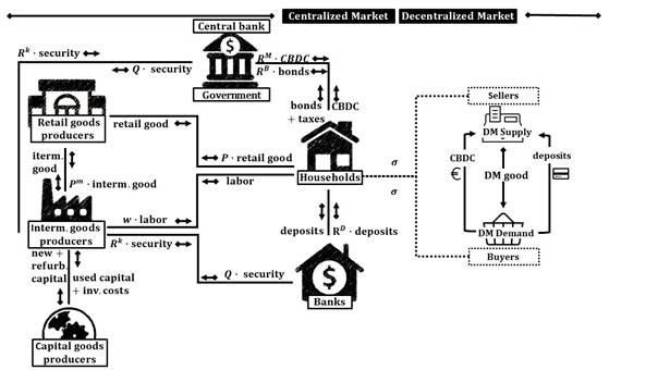
Figure 1: Overview of the model structure

While money in the CM is modeled as a store of value, the DM provides a role for money as a means of exchange. Households receive a preference shock at the beginning of the DM that determines whether they become sellers or buyers, creating a double-coincidence-of-wants problem. In the DM, households are anonymous and can either pay with bank deposits or with CBDC. Like Keister and Sanches (2023), we assume that sellers are endowed with a technology to recognise specific means of payment, i.e. CBDC or bank deposits, but that they cannot accept securities or other types of claims. In practice, this means that sellers have the technology, such as card readers, installed to accept CBDC or debit cards. This setup makes money essential and allows us to study the interactions between the central bank’s balance sheet, monetary policy and the payment function of money.

We first describe the decision problem of households, banks and different types of firms in the CM before we turn to the framework and the decision problems of buyers and sellers in the DM.

2.1 The centralised market (CM)

The CM features the usual New-Keynesian frictions that allow monetary policy to have real effects. Retail goods producers operate under monopolistic competition and repackage output produced by intermediate goods producers. Moreover, the model assumes Calvo-type sticky prices such that a firm can freely adjust its price with probability 1 - ? in a specific period whereas in all other periods it can only index its price to lagged inflation. In addition to these two frictions, the model includes investment adjustment costs for intermediate goods producing firms and an incentive constraint for bankers that creates a friction in the bank intermediation process. This financial friction magnifies the impact of shocks to banks’ net worth on the real economy and credit flows on the one hand while, on the other hand, it amplifies the effect of these shocks on the availability of deposits and thereby affects transactions in the DM. We will further discuss the financial sector and how this friction plays out below.

Households

In the CM, there is a continuum of identical households of measure unity. Each household has two different types of members: a fraction f of the household are bankers and a fraction 1 - f are workers. Bankers remain bankers in the next period with a time-independent probability ?. This implies that in each period (1 - ?)f bankers become workers and vice versa. In the CM, households maximise their utility by choosing consumption C_t^CM, labour L_t, real CBDC holdings M_t, real deposits D_t, and real bond holdings B_t, taking the expected continuation value in the DM, V_t^DM, into account. The households’ value function in the CM therefore is

(1)

with and s.t. the budget constraint

CtCM + Mt + Dt + Bt = wtLt - Tt + RtMM^t-1 + RtDD^t-1 + RtBBt-1 + ?t, (2)

where w_t is the real wage, T_t denotes lump-sum taxes, R_t^M, R_t^D and R_t^B are the gross real rates of return on CBDC, deposits and bonds, respectively, and ?_t is the net payout from the ownership of financial and non-financial firms, including the net cash-flow from trading state-contingent securities.⁶ While CBDC, deposits and bonds are all financial assets, only deposits and CBDC can be considered money as they can be used to carry out transactions in the DM. Bonds, by

⁵Like Aruoba and Schorfheide (2011) we abstain from modelling habit persistence, which simplifies calculations in the DM.

⁶Note that the budget constraint is expressed in real terms, i.e. in units of the CM consumption good. Consequently, M_t and D_t denote real CBDC and real deposit holdings. We discuss the price level and inflation later on.

contrast, serve as the benchmark asset against which the liquidity premium is measured.^[5]M^_t and D^_t are CBDC and deposit holdings that are carried over from the previous DM and depend on whether the household is a buyer, a seller or inactive in the DM, namely

for buyers for buyers

for sellers and for sellers otherwise ? otherwise

where m^B_t and d^B_t are CBDC and deposits spent and m^S_t and d^S_t are CBDC and deposits obtained in the DM (see Section 2.2). On aggregate, sellers receive the amount that buyers pay i.e. and . Since the households’ utility function is log-linear,

CBDC and deposit holdings are identical for all households at the end of the CM, irrespective of whether they were buyers, sellers or inactive in the DM. This feature makes the model tractable by ensuring that the optimality conditions do not depend on individual state variables.

Optimality conditions for the CM (Equations 3 and 4) require that the marginal utility of consumption in the CM, denoted by ?^CM_t , equals the marginal disutility of labour divided by the real wage ?/w_t. The marginal values of CBDC, deposits and bonds in the CM, and , reflect the costs of acquisition and their continuation values denoted by ,

.

(3)

for a_t = {M_t,D_t,B_t} (4)

The envelope conditions (Equation 5) state that the marginal values of assets in the CM depend on their interest payments, weighted by the marginal utility of consumption in the CM, implying that assets are valued only as store of value in the CM as transactions in the CM are not modelled explicitly. By contrast, in the DM money derives value only as a means of exchange because discounting and interest payments take place only when the CM opens in the next period but not between the CM and the DM.

(5)

In this way, the store-of-value and the means-of-exchange functions of money are modelled to pertain to two distinct markets. It should be noted, however, that an implicit transaction motive exists also in the CM. As regards the third, unit-of-account, function of money, CBDC and deposits serve as two different forms of money, denominated in the same unit of account.^[6]

Banks

Banks are active only in the CM. Bank j invests into shares of intermediate goods firms and funds itself by household deposits D_j,t and equity N_j,t. Its balance sheet can be written as

, (6)

where S_j,t^B are the financial claims of the intermediate goods producers that the bank holds and Q_t is their relative price. On the asset side of its balance sheet, the bank will only hold claims of the intermediate good producers as they yield a higher return than government bonds.^[7]Bank deposits are used as a means of payment in the DM. Shocks to the banks’ balance sheet thus will not only affect capital investment and production in the CM but also transactions in the DM.

Bankers maximise the expected discounted terminal net worth of their bank V_j,t

with ? being the probability that the bank continues its operations in the next period, ß?_t,t+1+i the stochastic discount factor that the bankers in period t apply to their earnings in t + i and the gross real return on the banks’ investment in the intermediate good producers. Making use of the balance sheet identity in Equation (6), is thus the net interest margin on the bank’s investment into the intermediate good firms.

Banks are subject to an incentive constraint that limits the amount of deposits the households are willing to entrust them with and therefore the amount of investment. Specifically, it is assumed that households can only recover a share 1 - ? of the bankers’ assets in case of a bankruptcy, see Gertler and Karadi (2011). To avoid that the banker prefers to divert a share ? from the funds invested in the project, the net worth of the bank, V_j,t, has to exceed the gain the banker can realise from such illicit diversion.

(8)

When the incentive constraint binds, the banks’ net worth constrains the amount of investment and deposits, implying that a shock to the banks’ net worth will spill over into investment and production.^[8]As in Gertler and Karadi (2011), our parametrisation ensures that the constraint always binds locally in the steady state.

Firms

The production sector follows Gertler and Karadi (2011) with a set-up that is standard in New Keynesian models. It consists of capital good producing firms, intermediate good producing firms and retail good selling firms.

Capital good firms operate in a competitive environment. They buy capital K_t from the intermediate good firms at the end of period t, repair depreciated capital and build new capital, and then resell it to the intermediate good firms. As the intermediate good firms face adjustment cost on net investments, capital good producers may earn profits outside of the steady state, which they distribute in lump-sum form to their owners, the households. The discounted profit for capital good producers is given by:

, (9)

in which I_t^N ? I_t - ?(U_t)?_tK_t is the net capital produced, I_t is the gross capital, ?(U_t) is the depreciation rate,^[9]U_t is capital utilisation, ?_t is a capital quality shock and I^SS is the level of investment in steady state. Following the literature, we assume quadratic flow adjustment costs on net investment (Christiano et al., 2005; Gertler and Karadi, 2011), with ? denoting a scaling parameter.

The competitive intermediate good firms, indexed by M, acquire capital K_t+1 at the end of period t for production in period t + 1. After production, they can sell the capital on the market to the capital good firms without adjustment cost. The capital choice problem of the intermediate good firms is therefore static. To fund capital, the firms issue equity S_t at a price Q_t such that Q_tK_t+1 = Q_tS_t.¹² Capital is mainly funded by banks that purchase capital securities S_t^B. Notwithstanding this, the central bank acquires capital securities S_t^CB to balance CBDC issuance on its balance sheet, such that in total S_t = S_t^B +S_t^CB. Production in the intermediate goods sector is given by

YtM = At (Ut?tKt)? L1t-? (10)

A_t denotes total factor productivity and ? the elasticity of substitution of capital in production. The competitive environment with zero profits implies that all ex-post returns of the intermediate good firms are paid out as a return on capital securities

(11)

where P_t^M denotes the price of the intermediate good.

The retail good firms use intermediate output as the sole input with a one-to-one input output ratio and operate in a monopolistically competitive setting that consists of a continuum differentiated retail firms of mass unity. . The final aggregated output on the CM, Y_t^CM, is a constant elasticity of substitution (CES) aggregate of the output , produced by retailer i and is given by

, (12)

where ? denotes the elasticity of substitution between goods produced by different retailers. Each period, retailers can reset their price to the optimal price P_t* with probability 1 - ?. The

?c = ?SS - b/(1+ ?) and the subscript SS indicating the respective steady state values.

12The intermediate good firms do not face any credit frictions in their funding because the credit friction in the model relates to the bank’s funding obtained from the households.

aggregate price level on the CM is therefore sticky and evolves according to

, (13)

where is the previous period’s inflation rate in the CM. Before discussing policy, we next describe the DM and its linkages with the CM.

2.2 The decentralised market (DM)

At the beginning of the DM, a fraction ? of households receive a business opportunity and become sellers of the retail good in the DM, whereas a fraction ? become buyers and a fraction (1-2?) do not participate in the DM.^[10]The value function in the DM before the determination of types is therefore a weighted average of the three possible outcomes:

(14)

where V_t^DM,B and V_t^DM,S denote the value of being a buyer or a seller in the DM and reflects the value of participating in the next CM, adjusted with the households’ discount factor between periods ß. To complete the households’ problem and to derive the optimality conditions given in Equation 3, we need to determine the marginal value of assets for buyers and sellers in the DM.

for a_t = {M_t,D_t,B_t} (15)

Buyers and sellers are matched one-to-one, assuming an efficient matching technology in the DM that matches every buyer with a corresponding seller. With respect to the pricing mechanism, we assume price taking as in Rocheteau and Wright (2005), which is more tractable than alternative pricing mechanisms.^[11]It keeps the double coincidence and the verifiability assumptions that make money essential in trading in the DM, although the price is set at the market-clearing level by a Walrasian auctioneer.^[12]A buyer derives concave utility U(C_t^DM) from consuming the DM good and faces the following optimisation problem:

(16)

with U(C_t^DM) = ?ln(C_t^DM) and s.t.

PtDMCtDM = mt + dt,

0 ? m_t ? ?_MM_t, (17)

0 ? d_t ? ?_DD_t.

Buyers maximise utility from DM consumption, which is assumed to be of the same functional form as CM consumption. ?_t captures the weight of DM consumption relative to CM consumption. While ?_t is constant in general, it can be subject to an aggregate preference shock which is analysed in Section 4.4. When choosing DM consumption, households take the depletion of their money holdings ahead of the next CM into account. Consumption in the DM is paid for with CBDC m_t and deposits d_t. Negative CBDC or deposit balances are not allowed. We assume that only a fraction 0 ? ?_M ? 1 and 0 ? ?_D ? 1 of total CBDC and deposits holdings can be spent in the DM. Transactions in the DM are thus constrained by disposable money balances, ?_MM_t and ?_DD_t, brought into the DM. The parametrisation of ?_M and ?_D reflects the assumption that a part of households’ spending constitutes relatively inelastic fixed expenses, such as rent, insurance, utilities or other bills, for which households want to keep precautionary balances when entering the next CM. Evidence from the ECB’s SPACE payment survey (European Central Bank, 2020) corroborates that households’ bill payments are sizeable and make up 75% of total payment values. ^[13]

Demand for the DM consumption good

We can derive the demand for the DM consumption good C_t^DM from the optimality conditions for buyers, which implies that the demand for goods in the DM satisfies

, (18)

where ?^m,l_t and ?^m,h_t are the Lagrange multipliers associated with the lower and upper constraints on CBDC holdings, i.e. on 0 ? m_t ? ?_MM_t.^[14]Buyers consume the DM good, C_t^DM, until their marginal utility of consumption in the DM, U_CtDM , equals the relative price of the DM good P_t^DM, multiplied by the marginal benefit of holding money, the expression in square brackets.

This term consists of the marginal value of money balances carried over into the next CM,

, and the liquidity benefit of money in the DM, captured by the Lagrange multipliers

that will be discussed in more detail below.

The buyers’ optimality condition (Equation 19) states that the interest rate spread between CBDC and deposits is determined by the difference in the shadow values of holding CBDC and deposits, where ?^d,l_t and ?^d,h_t are the Lagrange multipliers associated with the lower and upper constraints on deposit holdings:

. (19)

The sellers’ optimisation problem (Equation 20) balances the costs of producing the DM good Ct^DM against the benefits of holding higher money balances in the subsequent CM.

(20)

For tractability, the sellers’ production function is a concave function of their effort to produce the DM good. Unlike production in the CM, DM production does not require capital, yielding convex production costs for the DM good, which are assumed to take the form C(C_t^DM) =

?(CtDM)?1.

From the sellers’ optimality conditions we can derive a supply function for the DM good, which states that the relative price of the DM good equals the marginal cost of production C_tDM , divided by the discounted marginal value of money balances in the CM.

(21)

Combining the buyers’ demand and the sellers’ supply function yields the DM equilibrium condition:

. (22)

Money holdings and DM outcomes

Depending on the availability of money balances, two regimes can emerge in the DM: With sufficient liquidity, transaction constraints arising from money holdings do not bind (i.e. ?^m,l_t = ?^m,h_t = ?^d,l_t = ?^d,h_t = 0) and the optimal output in the DM is determined by the equality of the marginal utility of consumption and the marginal costs of production of the DM good.

^UCtDM* ⁼ CCtDM*. (23)

In the unconstrained case, DM output does not depend on CBDC and deposit balances. Consequently, an additional unit of money has no transaction value in the DM and interest rates on CBDC, deposits and bonds are equal: . By contrast, money balances do influence DM market outcomes if liquidity is scarce.

As long as CBDC and money balances are positive and DM consumption is valued by buyers, we can establish that in the constrained case only the upper bounds on CBDC and deposits will bind. Moreover, if the upper bound for either CBDC or deposits is binding, then the other upper constraint will bind as well (see Appendix B.1). The Lagrange multipliers ?^m,h_t and ?^d,h_t enter the marginal value of CBDC and deposits in the DM in Equation 24 and reflect the liquidity value of a marginal unit of money:

Vt,MDMt = ß?CMt+1 RtM+1 + ??M?m,ht = ?CMt Vt,DDMt = ß?CMt+1 RtD+1 + ??D?d,ht = ?CMt

(24)

The value of ?^m,h_t is determined by the optimality conditions of the buyers (Equation 18) and the sellers (Equation 21)

, (25)

whereas the value of ?^d,h_t is determined by Equation 19. The buyers’ constrained demand is then determined by their disposable money balances (Equation 16)

PtDMCDM = ?MMt + ?DDt. (26)

We can now write down the optimality conditions for money holdings represented by the Euler equations for CBDC and deposits:

(27)

(28)

In the constrained case, an additional unit of money enables higher DM consumption, which gives rise to a liquidity premium. This implies that interest rate on money lies below the interest rate on bonds that do not offer liquidity services. The expressions in square brackets in Equations 27 and 28 reflect the liquidity premia for CBDC and deposits, respectively. We assume that both forms of money, i.e. CBDC and deposits, are equally useful for transactions in the DM and therefore perfect substitutes.^[15]Specifically, the relative marginal utility of being able to increase DM consumption is weighted with the probability of becoming a buyer, ?, and the fraction of money that can be spent in the DM, ?. The closer households are to their optimal DM consumption, the smaller is the liquidity premium. A small liquidity premium signals that monetary exchange is very effective. When DM consumption is at its optimal level,

U_CtDM = CCtDM , the liquidity premium becomes zero (i.e. the term in the square brackets is unity). In this situation, money carries the same interest as bonds with

and there is no additional money demand for transaction purposes. In this way, the Euler equation features a smooth transition from the constrained to the unconstrained region.

2.3 Government and aggregation of DM and CM

We now specify the actions of the government and set out how we aggregate outcomes in the CM and the DM. The government spends an exogenous amount, G. Furthermore, it issues bonds B_t, covers any profits or losses of the central bank ( ) and taxes households or pays transfers to them, T_t, leading to the following government budget constraint:

G + R_t^BB_t-1 = B_t + T_t^CB + T_t (29)

We now turn to aggregating real output and inflation across the CM and the DM. The household optimisation problem is defined in real terms, with the CM consumption good C_t^CM as the numeraire. The combined real output in both markets is

Yt = YtCM + YtDM

(30)

= CtCM + It + Gt + f(·)(ItN + ItSS) + ?PtDMCtDM

with Y ^DM = ?P_t^DMC_t^DM. DM output, >_DM, is calculated by adjusting production in the DM with the relative price between the CM and the DM good, P_t^DM, and the probability to consume in the DM, ?. We follow Aruoba and Schorfheide (2011) in defining economy-wide inflation by a Fisher price index, weighting the size of each market with its steady state share:

(31)

where s* is the steady state share of the DM market, and

since P_t^DM is expressed in relative CM prices. The aggregate (CM

and DM) price level therefore evolves according to

t

Pt = P0 ?(??CM)1-s* (??DM)s*

?=1

2.4 Central bank

The central bank has two policy instruments. It sets the interest rate on government bonds and affects the interest rate on money by issuing CBDC. In this way, the central bank can use two instruments, which work through different channels, to affect the economy. By setting the interest rate on government bonds, it determines the attractiveness of assets as a store of value, whereas by setting the interest rate on CBDC, it influences the means-of-exchange function of money in the DM.

The central bank sets the nominal interest rates on government bonds, , according to a standard Taylor rule

(32)

where i^B* is the steady state interest rate and ? is a smoothing parameter. The rule considers aggregate inflation and the aggregate output gap, which is defined as

^Y_tgap = (^Y_tCM,gap)1-s*(^Y_tDM,gap)s*

Note that M_t and D_t denote real CBDC and real deposit holdings. All gross rates of return,

and , are also defined in real terms. Real and nominal interest rates are linked by the Fisher equation for a = {M,D,B}. CBDC is issued following an interest rate rule of the form

(33)

According to this rule, the central bank issues CBDC to target the liquidity premium, which we define as the spread between the interest rates on bonds and money A liquidity premium on money results in a positive spread for since, compared to bonds, money has a value as a means of payments in the DM, implying that the interest rate on money lies below the interest rate on bonds that function only as a store of value. When liquidity is abundant, the central bank issues a fixed base amount of CBDC M_t^S = m. In this case, i^M_t = i^B_t and there is no liquidity premium. The more CBDC demand exceeds the base issuance (M_t-m), however, the higher the liquidity premium becomes because money becomes more valuable as a means of transactions, which translates into a low . The central bank then issues more CBDC, but at an increasingly unattractive interest rate in order to reduce the spread relative to its steady state value. This can be seen by rewriting Equation 33 as a money supply rule:

(34)

As CBDC and deposits are perfect substitutes, the central bank determines both, i_D and i_M, by setting the interest rate on CBDC. The CBDC rule implies that, when faced with a high deposit rate and a compressed liquidity premium, the central bank decreases CBDC issuance.

¹⁹Section 4.5 and Appendix A discuss different parametrisations of this rule.

A high deposit rate indicates stressed bank funding conditions and low deposit holdings. In such a situation, a decrease in CBDC supply increases the transaction value of money and leads to a higher liquidity premium by lowering i_M. This causes a corresponding decrease in i_D and thereby eases banks’ funding costs. In addition, a decrease in CBDC supply crowds in deposits as households substitute CBDC for deposits. The CBDC rule thus stabilises the economy through a stabilisation of bank funding conditions in the face of financial stability shocks.

The model setup abstracts from cash, reserves and other central bank liabilities. Therefore,

CBDC issuance lengthens the central bank’s balance sheet. We assume that, in order to issue CBDC, the central bank purchases an equivalent amount of capital securities S_t^CB.^[16]

Mt = QtStCB (35)

Profits or losses of the central bank are distributed via lump-sum transfers T_t^CB to the government. The budget balance of the central bank is accordingly:

(36)

3 Calibration and shocks

Table 1 documents the parameter values for the numerical simulation. We calibrate the model such that one period represents a quarter. For the CM, we take most values from (Gertler and Karadi, 2011, henceforth GK11) and adapt some parameters to euro area data. To keep the model tractable, a unitary labour elasticity is required. Although this affects the results quantitatively, we checked that the impulse responses remain qualitatively unchanged. To approximate the increasing marginal cost of labour in GK11, we follow Aruoba and Schorfheide (2011) and set the utility weight of labour to their estimated value of 24.3 (instead of 3.409 in GK11). In addition, we set government spending G to 48% of steady state output, which is the average share of total government expenditure to GDP for euro area countries between

2004-2021. To better fit investment adjustment costs ? to euro area values, we set ? = 4.5 as in Maih et al. (2021). Moreover, we align the probability of keeping prices fixed with the value of

0.84 in the ECB’s New Area Wide Model, from which we also take the Taylor rule output and inflation coefficients of 2.74 and 0.03, respectively (Coenen et al., 2018).

For the calibration of the DM, we follow Aruoba and Schorfheide (2011) in setting the share of households engaging as sellers or buyers in the DM ? = 0.295. The other parameters for the DM are informed by euro area payment data. We set the payment fraction of deposits and CBDC to ?_D = ?_M = 25.14%, which according to the euro area SPACE survey (European Central Bank, 2020) is the share of payments not accounted for by bill payments. Equality of ?_M and ?_D implies that we assume they feature similar transaction convenience on aggregate.^[17]

The relative utility weight of DM consumption is set to ? = 4.35 to target a liquidity premium of 1.4% p.a. in the model version with CBDC, which corresponds to the average difference between the interest rate on the ECB’s main refinancing operations (MRO) and the rate on euro area overnight deposits between 2000-2016.^[18]Overall, this results in a share of DM consumption to total consumption of 55% which equals the share of point-of-sale and peer-to-peer transactions to all transactions (i.e. including bill payments) in the euro area (European Central Bank, 2020).

We calibrate parameters of the CBDC interest rate rule to result in a steady state share of CBDC to total money (CBDC and deposits) of 15.8%, which is the 2000-2016 average euro area share of currency in circulation to M1. For this, we set the CBDC interest rate reaction to the liquidity premium to ?_m = 0.02444.^[19]By calibrating CBDC issuance in steady state to the share of currency in circulation we assume that in the steady state CBDC performs an equivalent role as cash does in today’s economy.²⁴ We set the CBDC issuance in the absence of a liquidity premium (i.e. for the unconstrained DM) as small as possible with m— = 0.0002, which implies that payment needs are fully satisfied by the amount of deposits that banks provide and additional liquidity is not needed. In our model, CBDC will crowd out bank deposits because both means of payment are perfect substitutes. At the same time, the central bank can determine the extent to which bank deposits are shifted into CBDC in the steady state by choosing its reaction parameter ?_M in the CBDC rule. This choice, however, will have implications for the stabilisation properties of CBDC as a monetary policy tool.^[20]

We analyse seven different types of shocks that we group into four categories: monetary policy shocks, business cycle shocks, financial shocks and shocks to the liquidity premium. First, we investigate two monetary policy shocks, namely a contractionary conventional monetary policy shock to the Taylor rule that increases by 50 basis points and a shock to the CBDC interest rate rule that raises by 50 basis points on impact. To investigate business cycle dynamics, we study a 1% shock to total factor productivity (TFP) A_t. For the financial shocks, which correspond to the shocks analysed in GK11, we examine a deterioration in the quality of capital ?_t of 5% and a 1% shock to banks’ net worth N_t. We further look at shocks to the liquidity premium, which we model as a disturbance to the usefulness of deposits for payments (i.e. a 5% payment technology shock to ?_D) and a 5% increase in the preference for DM consumption ?. All shocks follow an AR(1) process, e_i,t = ?_ie_i,t-1-?_i,t with shock type i = {i^M,i^B,A,?,?,?_D}.

Parameter	Value	Description
Households ß	0.990	Discount factor
?	24.3	Relative utility weight of labour
?	4.35	Relative utility weight of DM consumption
?	0.295	Probability of being a buyer or seller in the DM
?	0.68	Effort elasticity of DM good production
?D	0.2514	Share of deposits available for DM transactions
?M	0.2514	Share of CBDC available for DM transactions
Banks ?	0.972	Survival probability of bankers
?	0.381	Fraction of capital that can be diverted
?	0.002	New banks’ endowment fraction
Firms ?	0.33	Elasticity of capital demand
?	4.5	Scaling parameter investment adjustment costs
?	7.2	Elasticity of marginal depreciation w.r.t. utilisation rate
?	4.167	Elasticity of substitution between goods

Continued on next page

? 0.82	Probability of keeping prices fixed
?p 0.241 Policy parameters	Price indexation of inflation
?? 2.74	Taylor rule inflation coefficient
?y 0.03	Taylor rule output coefficient
?M 0.02444	CBCB rule coefficient
m 0.0002 Shock parameters	CBDC base issuance
?iM 0.2	Persistence of CBDC rule shock
?iB 0.2	Persistence of monetary policy shock
?a 0.95	Persistence of TFP shock
?? 0.66	Persistence of capital quality shock
?? 0.96	Persistence of DM preference shock
??D 0.9	Persistence of payment technology shock

Table 1: Calibration of parameter values

4 Responses to macroeconomic shocks

In this section, we analyse how the presence of a CBDC changes the dynamic responses to the different shocks compared to a model setup with deposits as the only means of exchange. By comparing responses of macroeconomic variables to these shocks with and without a CBDC, we can analyse the transmission channels and the role of a CBDC as an additional monetary policy tool in the New Monetarist New Keynesian model.

We find that the central bank can affect the transmission of shocks by varying the interest rate on money relative to government bonds since CBDC and deposits are valued as a means of exchange in the DM and therefore carry a liquidity premium. In our model, CBDC and deposits are perfect substitutes, as both are equally useful for transactions in the DM. Consequently, their interest rates are always identical and only their relative quantities adjust to shocks hitting the economy. In the steady state, coexistence of CBDC and deposits is ensured by our calibration of ?_M, which results in steady state shares of 15.8% for CBDC and 84.2% for deposits.

The liquidity premium affects the economy through two main channels. The supply of CBDC directly affects consumption on the DM by making money more or less scarce. It also affects bank funding conditions and thereby influences the profitability of investments. As in George et al. (2020), we find that the existence of CBDC allows the central bank to target fluctuations in the liquidity premium and thereby opens up a second channel through which monetary policy can influence output and inflation.

4.1 Monetary policy shocks

Figure 2 shows the responses to a CBDC rule shock that increases i^M by 50 basis points (bottom middle panel). Because CBDC and deposits are perfect substitutes, i^D rises by the same amount and the liquidity premium on money decreases. The shock crowds out some bank deposits. By increasing i^M via the CBDC rule, the central bank increases its issuance of CBDC, which it offsets by purchasing capial securities QS^CB. This has a positive effect on gross investment as the increase in CBDC exceeds the fall in deposits. Although the higher CBDC supply crowds out some deposits, it stimulates consumption, mostly in the DM, as the increased availability of money enables more transactions. This leads to a sharp rise in inflation, to which the central bank reacts via the Taylor rule by increasing the government bond rate, which dampens investment. As the shock to the CBDC rule recedes, CBDC supply falls back to its steady state level, deposits increase, and interest rates and the liquidity premium return to steady state values as well.

This exercise shows that through the provision of CBDC, the central bank can affect output and inflation by setting the liquidity premium on money. By modelling the transactions value of money explicitly, our model thus allows us to study additional transmission effects that run through both, the liquidity premium and the funding effects of CBDC.

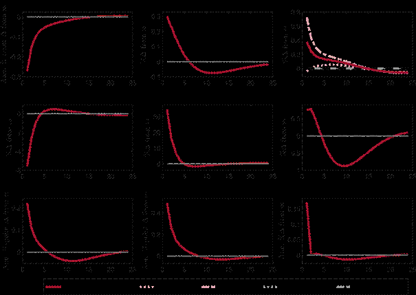
Figure 2: Responses to a 50 bps CBDC rule shock with CBDC

Next, we turn to the responses of a contractionary monetary policy shock to the Taylor rule that increases i^B by 50 bps. Figure 3 shows the responses for the case with a CBDC as well as without a CBDC, i.e. when deposits are the only means of payments in the economy. An increase in the government bond rate also raises i^M and i^D through the households’ optimality conditions (Equations 27 and 28). A higher bond rate can be interpreted as a shock to the store-of-value function of money, which leads to a decrease in consumption and investment. Output falls, implying a lower supply of consumption goods in the DM, which lowers the liquidity premium on money as less means of payments are required for transactions on the DM. In the presence of a CBDC, the central bank reacts to the fall in the liquidity premium by reducing the supply of CBDC, which crowds in deposits and mitigates the increase in i^M, i^D and i^B as well as the fall in the liquidity premium.

Overall, the effects of a monetary policy shock on inflation are almost identical with and without a CBDC.^[21]For consumption and investment, the presence of a CBDC tends to reduce the amplitude of the fluctuations somewhat without changing qualitatively the pattern of the response. The reason for this is that via its CBDC rule the central bank lowers the CBDC supply, mitigates the fall in the liquidity premium and eases bank funding strains by crowding in deposits. We conclude that monetary policy remains equally effective in the presence of a CBDC while it reduces fluctuations in interest rates and real variables, rendering monetary policy transmission smoother than without a CBDC.

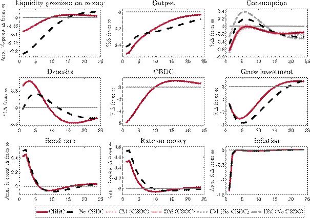
Figure 3: Responses to a contractionary 50 bps monetary policy shock with and without CBDC

4.2 Business cycle shocks

Turning to business cycle shocks, we investigate a shock to total factor productivity that we interpret as a negative supply shock.^[22]Figure 4 shows the responses with and without CBDC.

The decline in TFP reduces output, investment and consumption in the CM. The productivity shock spills over into the DM, leading to a decline in DM consumption, a lower demand for money and a decrease in the liquidity premium. According to its CBDC rule, the central bank reacts to the fall in the liquidity premium by reducing CBDC supply, which leads to an increase in deposits, being a perfect substitute for CBDC, and a rise in i^M and i^D, which mitigates the drop in the liquidity premium. As the liquidity premium declines less in the presence of a CBDC, DM consumption falls more than without a CBDC since the reduction in CBDC supply is not fully offset by the increase in deposits. Overall, the reaction of inflation to a TFP shock is dampened by the presence of a CBDC. Prices in the DM fall more strongly because DM demand is dampened by the impact of the CBDC rule whereas inflation in the CM is basically the same with and without CBDC, leading to smaller aggregate fluctuations in inflation in the presence of a CBDC. Owing to the increase in deposits with a CBDC, bank funding conditions improve and investment recovers faster than without a CBDC, leading to a faster recovery in output. We thus find that the presence of a CBDC allows the central bank to stabilise the economy in the face of a supply shock more effectively as it can influence economic outcomes through a second channel that operates through the liquidity premium.

The central bank reacts to an increase in the liquidity premium and expands CBDC supply, which leads to a drop in deposits. Except for CBDC and deposits, reactions in the model with and without CBDC are virtually identical, so that we refrain from showing the impulse responses.

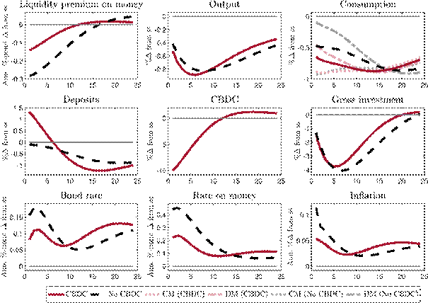
Figure 4: Responses to a 1% TFP shock in the NMNK model with and without CBDC

4.3 Financial shocks

Next, we analyse how, in the presence of a CBDC, the economy reacts to financial shocks, namely a capital quality shock and a shock to banks’ net worth. Overall, we find that the output response tends to be dampened with a CBDC for a capital quality and a bank net worth shock, while the inflation response is similar for the capital quality shock and somewhat less volatile for the bank net worth shock.

Figure 5 shows the response to a decline in capital quality with and without a CBDC. The capital quality shock lowers the price of capital securities that banks hold on the asset side of their balance sheet and curtails their lending. As the shock lowers the effective capital stock, production is reduced and investment, consumption, and output all decline. The shock tightens banks’ leverage constraints, triggering a reduction in deposits to deleverage. At the same time, the large decline in consumption reduces the demand for money more than the decline in deposits, so that without a CBDC the liquidity premium falls. In the case with a CBDC, the central bank stabilises the decline in the liquidity premium by issuing CBDC according to the CBDC rule. This dampens the impact of the shock on output, consumption and investment but leads to a larger decline in deposits as households replace deposits with CBDC. Yet, by issuing CBDC against the purchase of capital securities, the central bank lowers the cost of investment and dampens the investment response. This translates into a less pronounced and smoother decline in output and a smaller decline in consumption. The inflation response with and without CBDC is very similar.

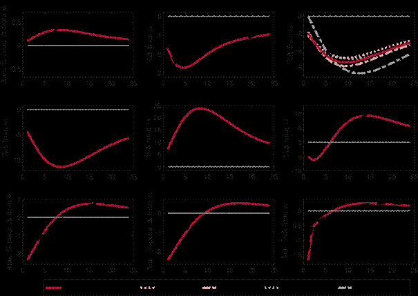
Figure 5: Responses to a negative 5% capital quality shock with and without CBDC

Figure 6 shows the responses to a 1% decline in banks’ net worth, which is redistributed to households as in GK11. Similar to the the capital quality shock, the presence of a CBDC helps to contain fluctuations in output and inflation following a negative shock to banks net worth.

In a frictionless model, this redistribution should not have any effects on the economy as total wealth remains constant and is only shifted from household members that are bankers to those that are workers. Owing to the frictions in the CM (in GK11 and our model) this shock reduces the liability side of banks’ balance sheets, which forces banks to curtail lending, leading to a contraction in investment. At the same time, banks have increased funding needs, which leads to an increase in deposits and the interest rate on money. As production declines only gradually, consumption on impact increases, in particular in the DM as more money is available, as is also evident from the fall in the liquidity premium. Over time, output declines on account of the lower capital stock resulting from the decline in investment and consumption. Interest rates and deposits decline as well. In the presence of a CBDC, the central bank reacts to the decrease in the liquidity premium by lowering CBDC supply. Part of the lower supply is replaced by deposits, which benefits bank funding conditions and dampens the investment response. Owing to the smaller expansion of money supply, consumption in the DM increases less than in the case without a CBDC. Overall, the presence of a CBDC leads to a less persistent and less pronounced output decline and less volatility in inflation.

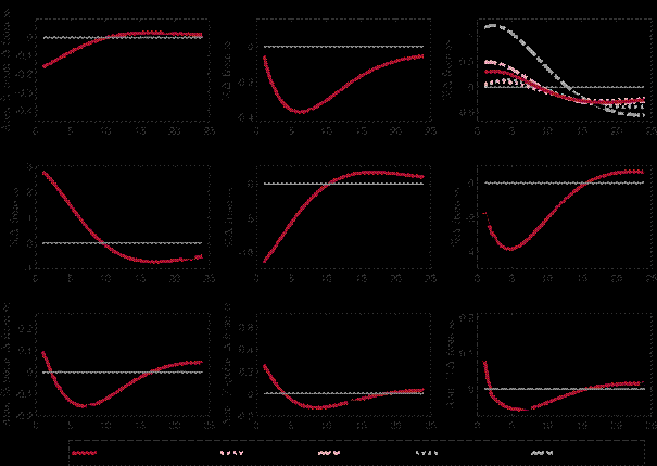
Figure 6: Responses to a negative 1% bank net worth shock with and without CBDC

4.4 Liquidity premium shocks

This section focuses on shocks that can only be studied in a model with an explicit modelling of the means-of-exchange function of money, namely a payment efficiency and a DM preference shock. While both shocks lead to a rise in the liquidity premium, their impact on consumption differs and therefore also their overall impact on output and inflation. With a CBDC, their responses are less pronounced for a payment efficiency shock but more pronounced in response to a DM preference shock.

Figure 7 presents the responses to a drop in the payments efficiency of deposits by 5%, modelled as a shock to the fraction of deposit holdings that can be spent in the DM, ?_D. When there is no CBDC available, consumption in the DM declines as households can transact less with the deposits they own. At the same time, deposits have a higher value as a means of exchange, leading to a rise in the liquidity premium. While the amount of deposits remains broadly unchanged, bank funding conditions improve as the rate on deposits falls, which stimulates investment. Output falls on impact because the decrease in consumption exceeds the surge in investment but increases over time as consumption starts to recover. With a CBDC, the shock to the payment efficiency of deposits triggers an increase in CBDC supply as the central bank reacts to the rise in the liquidity premium. As a response, households shift into CBDC and deposits decline. CBDC issuance stabilises the liquidity premium and dampens the effect on DM consumption. Investment increases less and is affected through several channels: a higher demand for capital securities S^CB via the central bank’s CBDC issuance, a lower demand for S^B as bank funding conditions worsen, and lower interest rates as conventional monetary policy reacts to the decrease in inflation that results from lower DM consumption.

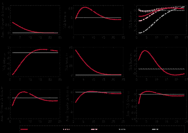
Figure 7: Responses to a 5% reduction in the payment efficiency of deposits with and without

CBDC

Figure 8 shows the responses to a 5% increase in the preference for consuming the DM good. Aruoba et al. (2011) interpret this shock as a money demand shock, which increases the transaction demand for money. As banks’ deposits issuance is limited by the leverage constraint, the liquidity premium increases. When there is no CBDC, the increase in the liquidity premium reduces the cost of bank funding, which leads to a rise in investment. Consumption in the DM increases whereas it falls in the CM. Driven by the rise in investment, output increases, which is reflected in a further rise in consumption in both, the CM and the DM. Inflation rises as well, which triggers a monetary policy reaction in i^B that eventually brings output and inflation back to their steady state values. In the presence of a CBDC, the central bank satisfies a part of the increased demand for money. Deposits fall as the supply of CBDC increases and households replace part of their deposits with CBDC. Consumption in the DM increases even more with the expansion of the money supply. As the central bank reduces the increase in the liquidity premium by supplying CBDC, bank funding conditions improve less in response to the money demand shock than without a CBDC. The response of investment in the first few quarters after the shock is fairly similar as the reduction in deposits and the smaller decrease in bank funding costs are offset by higher asset purchases of the central bank accommodating the higher CBDC demand. Overall, with CBDC the increase in output is more pronounced but less persistent which is also reflected in a more pronounced and less persistent inflation response.

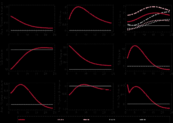
Figure 8: Responses to a 5% preference shock for DM consumption with and without CBDC

4.5 Insights from alternative model specifications

The explicit modelling of CBDC issuance and the integration of New Monetarist features into a New Keynesian model allows for analysing additional research questions. While not all of these can be pursued within the scope of the paper, this section summarises main insights from alternative modelling choices, which are presented in more detail in Appendix A.

Variation of the CBDC rule reaction parameter: In our baseline calibration, CBDC issuance reacts moderately to changes in the liquidity premium with the reaction parameter calibrated to match the steady-state share of currency in circulation.^[23]A higher reaction parameter in the CBDC rule better stabilises the liquidity premium but implies an increasing steady-state share of CBDC in the economy. Appendix A.1 shows impulse responses for a high and a low reaction parameter in the CBDC rule. As expected, with a high reaction parameter, the liquidity premium is stabilised more, which increases the stabilisation potential of CBDC but comes at the cost of larger fluctuations in deposits and a larger balance sheet of the central bank. By choosing a low reaction parameter, the central bank thus implicitly puts more weight on financial stability and bank funding costs and limits its footprint in the capital securities market. At the same time, it foregoes some of the stabilisation opportunities that the CBDC rule allows for. The lower the CBDC rule parameter, the more the reaction to macroeconomic shocks resembles the case without a CBDC.

Comparison to a money in the utility function specification: Modelling the use of money as a means of payment explicitly comes at the price of additional complexity compared to an additively separable money in the utility function (MIU) specification that simply presumes a convenience yield of money. In Appendix A.2, we examine the insights provided by the explicit formulation of the means-of-exchange function. Overall, this exercise demonstrates that the additively separable MIU specification misses important dynamics. In the MIU model, the exogenous specification of liquidity convenience in the utility function also leads to a liquidity premium. However, in this way the liquidity function of money is less entwined with the core model mechanisms. Using a calibration that ensures a comparable steady state baseline in both model variants, the liquidity premium fluctuates substantially less in response to shocks than in the New Keynesian New Monetarist model. Importantly, the liquidity premium shows a much lower variance than what data suggest, which exhibit a standard deviation of 1.06 percentage points over the period from 2000-2016.^[24]The low variation in the liquidity premium leads to smaller fluctuations in CBDC issuance and except for the shock to the payment efficiency of deposits to less stabilisation of output and inflation.

However, further investigation is needed to compare the empirical validity of both specifications. For instance, Aruoba and Schorfheide (2011) find that monetary frictions are empirically relevant and of similar magnitude as New Keynesian frictions. Nonetheless, using US postwar data, the goodness-of-fit of the estimated MIU specification with separable utility performs somewhat better than the search-based specification.

Neutralising effects from the expansion of the central bank balance sheet: Since we abstract from other central bank liabilities than CBDC, CBDC issuance will always lengthen the central bank balance sheet as CBDC issuance cannot be funded by changing the composition of central bank liabilities. As CBDC holdings cannot substitute for cash or excess reserves on the liability side of the central bank balance sheet it automatically leads to an lengthening of the balance sheet. Therefore, the type of asset acquired by the central bank as a counterposition for CBDC issuance will matter for how CBDC issuance affects the economy. In our framework, the central bank balances CBDC issuance by purchasing capital securities, thereby directly stimulating asset prices and investment. Alternatively, the central bank could increase lending operations to banks or purchase government bonds, which would affect the economy through bank lending or the government spending and taxation. In Appendix A.3, we assume that the central bank purchases a government liability that cannot be held by any other agent in the economy and the government distributes the proceeds in a lump-sum manner to households in order to make CBDC issuance as neutral as possible with regard to the affects arising from the asset side of the central bank balance sheet expansion. Overall, with a neutral asset side the responses to business cycle shocks remain similar and mostly lie in between the results from the baseline model with and without a CBDC. This exercise demonstrate that partial equilibrium analysis focusing solely on the liability side of the central bank balance sheet neglects important implications on the economy that derive from the counterposition to CBDC issuance.

5 Conclusions

In this paper, we integrate a decentralised market in the spirit of Lagos and Wright (2005) into a Gertler and Karadi (2011) New Keynesian DGSE model with financial frictions, following the approach by Aruoba and Schorfheide (2011). In the decentralised market, money in the form of either bank deposits or CBDC is required to purchase consumption goods. In the standard New Keynesian centralised market, banks’ credit provision together with the supply of deposits is restricted by a leverage constraint. By simultaneously modeling the means-of-exchange and the store-of-value function of money, we are able to analyse the transmission of monetary policy, business cycle and financial shocks as well as shocks to the means-of-exchange function of money in the presence of an interest bearing CBDC.

By providing CBDC, the central bank affects the availability of money, thereby influencing the liquidity premium and the efficacy of exchange. On the one hand, the central bank sets the interest rate on bonds according to a standard Taylor rule, which determines the opportunity cost of money and thereby affects the demand for both, deposits and CBDC. This rule defines the margin between money and bonds holdings and thus can be interpreted as influencing the store-of-value function of money. On the other hand, the existence of CBDC gives rise to a second policy rule that allows the central bank to influence the liquidity premium and thereby affects the efficacy of exchange, i.e. the means-of-payment function of money. The interaction of the liquidity premium with money holdings and bank funding condition links the centralised with the decentralised market and gives rise to rich dynamics.

Overall, we find that a CBDC does not significantly alter the responses of the economy to the usual shocks but tends to smooth transmission. In particular, monetary policy shocks to a conventional Taylor rule generate similar responses of output and inflation with and without the presence of a CBDC, suggesting that monetary policy transmission is not impaired. In our model, the existence of a CBDC opens up a second channel for the central bank to influence the economy by stabilising the liquidity premium, which helps smooth and dampen consumption and investment responses. This allows the central bank to separately affect the store-of-value and the means-of-exchange function of money. Regarding shocks to the liquidity premium, a CBDC stabilises the responses of output and inflation if such shocks affect money supply but amplifies them if money demand is impacted. The dynamic impact of a CBDC on the economy depends on the degree to which the central bank adjusts CBDC supply to changes in the liquidity premium. The less the central bank counteracts changes in the liquidity premium, the more the dynamic reactions to macroeconomic shocks resemble the case without a CBDC. Moreover, we show that the impact of CBDC issuance on the economy originates from both, the liability and the asset side of the central bank balance sheet.

Analysing transmission in the presence of a CBDC in a New Monetarist New Keynesian model allows for an explicit modelling of the different functions of money, which opens up new transmission channels of monetary policy through the banking sector. It would be interesting to study these transmission channels in more detail, which would require a more elaborate modelling of the financial sector, including for instance, modelling interbank lending, central bank credit provision and collateral policies. We leave this for future research.

References

Adalid, R., Á. Álvarez-Blázquez, K. Assenmacher, L. Burlon, M. Dimou, C. López-Quiles, N. M. Fuentes, B. Meller, M. Munoz, P. Radulova, C. R. d’Acri, T. Shakir, G. Šílová, O. Soons, and A. Ventula Veghazy (2022). Central bank digital currency and bank intermediation. ECB Occasional Paper (2022/293).

Ahnert, T., K. Assenmacher, P. Hoffmann, A. Leonello, C. Monet, and D. Porcellacchia (2022).

The economics of central bank digital currency. ECB Working Paper No 2713.

Ahnert, T., P. Hoffmann, A. Leonello, and D. Porcellacchia (2023). CBDC and financial stability. ECB Working Paper No 2783.

Ahnert, T., P. Hoffmann, and C. Monet (2022). The digital economy, privacy, and CBDC. ECB Working Paper No 2662.

Andolfatto, D. (2021). Assessing the impact of central bank digital currency on private banks. The Economic Journal 131(634), 525540.

Aragao, M. A. T. (2021). A few things you wanted to know about the economics of CBDCs, but were afraid to model: a survey of what we can learn from who has done. Working Paper 554, Banco Central do Brasil.

Aruoba, S. B. and F. Schorfheide (2011). Sticky prices versus monetary frictions: An estimation of policy trade-offs. American Economic Journal: Macroeconomics 3(1), 6090.

Aruoba, S. B., C. J. Waller, and R. Wright (2011). Money and capital. Journal of Monetary Economics 58(2), 98116.

Assenmacher, K., A. Berentsen, C. Brand, and N. Lamersdorf (2021). A unified framework for CBDC design: Remuneration, collateral haircuts and quantity constraints. ECB Working Paper 2578, European Central Bank.

Auer, R., J. Frost, L. Gambacorta, C. Monnet, T. Rice, and H. S. Shin (2022). Central bank digital currencies: motives, economic implications and the research frontier. Annual review of economics 14, 697721.

Barrdear, J. and M. Kumhof (2022). The macroeconomics of central bank digital currencies.

Journal of Economic Dynamics and Control 142.

Bitter, L. (2020). Banking crises under a central bank digital currency (CBDC). Beiträge zur Jahrestagung des Vereins für Socialpolitik 2020.

Boar, C. and A. Wehrli (2021). Ready, steady, go? Results of the third BIS survey on central bank digital currency. BIS Papers (No 114).

Brunnermeier, M. K. and D. Niepelt (2019). On the equivalence of private and public money. Journal of Monetary Economics 106, 2741.

Burlon, L., C. Montes-Galdon, M. A. Munoz, and F. Smets (2022). The optimal quantity of CBDC in a bank-based economy. ECB Working Paper No. 2689.

Böser, F. and H. Gersbach (2020). Monetary policy with a central bank digital currency: The short and the long term. CEPR Discussion Paper No. DP15322.

Carapella, F. and J. Flemming (2020). Central bank digital currency: A literature review. FEDS Notes November 9, Board of Governors of the Federal Reserve System.

Chapman, J., J. Chiu, M. Davoodalhosseini, J. H. Jiang, F. Rivadeneyra, and Y. Zhu (2023). Central bank digital currencies and banking: Literature review and new questions. Bank of Canada Staff Discussion Papers (2023-4).

Chiu, J., M. Davoodalhosseini, J. H. Jiang, and Y. Zhu (2019). Central bank digital currency and banking. Staff Working Paper 2019-20, Bank of Canada.

Christiano, L., M. Eichenbaum, and C. Evans (2005). Nominal rigidities and the dynamic effects of a shock to monetary policy. Journal of Political Economy 113(1), 145.

Coenen, G., P. Karadi, S. Schmidt, and A. Warne (2018). The New Area-Wide Model II: an extended version of the ECB’s micro-founded model for forecasting and policy analysis with a financial sector. ECB Working Paper No 2200.

European Central Bank (2020). Study on the payment attitudes of consumers in the euro area (SPACE).

Fernández-Villaverde, J., D. Sanches, L. Schilling, and H. Uhlig (2021). Central bank digital currency: Central banking for all? Review of Economic Dynamics 41, 225242. Special Issue in Memory of Alejandro Justiniano.

Ferrari Minesso, M., A. Mehl, and L. Stracca (2022). Central bank digital currency in an open economy. Journal of Monetary Economics 127, 5468.

Fraschini, M., L. Somoza, and T. Terracciano (2021). Central bank digital currency and quantitative easing. Swiss Finance Institute Research Paper (21-25).

Garratt, R., J. Yu, and H. Zhu (2021). How central bank digital currency design choices impact monetary policy pass-through and market composition. Available at SSRN: https://ssrn.com/abstract=4004341.

George, A., T. Xie, and J. D. A. Alba (2020). Central bank digital currency with adjustable interest rate in small open economies. Policy research paper series, Asia Competitiveness

Institute.

Geromichalos, A. and L. Herrenbrueck (2022). The liquidity-augmented model of macroeconomic aggregates: A New Monetarist DSGE approach. Review of Economic Dynamics 45, 134167.

Gertler, M. and P. Karadi (2011). A model of unconventional monetary policy. Journal of Monetary Economics 58(1), 1734.

Gross, J. and J. Schiller (2021). A model for central bank digital currencies: implications for bank funding and monetary policy. Working paper available at SSRN 3721965.

Group of Central Banks (2020). Central bank digital currencies: foundational principles and core features. Report 1, Series of collaborations from a group of central banks.

Group of Central Banks (2021). Central bank digital currencies: financial stability implications.

Report 4, Series of collaborations from a group of central banks.

Gu, C. and R. Wright (2016). Monetary mechanisms. Journal of Economic Theory 163, 644657.

Herrenbrueck, L. (2019). Interest rates, moneyness, and the Fisher equation. 2019 meeting papers 1409, Society for Economic Dynamics.

Jiang, J. H. and E. Shao (2020). The cash paradox. Review of Economic Dynamics 36, 177197.

Kareken, J. and N. Wallace (1981). On the indeterminacy of equilibrium exchange rates. The Quarterly Journal of Economics 96(2), 207222.

Keister, T. and C. Monnet (2022). Central bank digital currency: Stability and information. Working Paper 22.03, Study Center Gerzensee.

Keister, T. and D. Sanches (2023). Should central banks issue digital currency? The Review of Economic Studies 90(1), 404431.

Kim, Y. S. and O. Kwon (2023). Central bank digital currency, credit supply, and financial stability. Journal of Money, Credit and Banking 55(1), 297321.

Kosse, A. and I. Mattei (2022). Gaining momentum results of the 2021 BIS survey on central bank digital currencies. BIS Papers 12514.

Lagos, R. and R. Wright (2005). A unified framework for monetary theory and policy analysis. Journal of Political Economy 113(3), 463484.

Maih, J., F. Mazelis, R. Motto, and A. Ristiniemi (2021). Asymmetric monetary policy rules for the euro area and the US. Journal of Macroeconomics 70, 103376.

Niepelt, D. (2020). Monetary policy with reserves and CBDC: Optimality, equivalence, and politics. CEPR Working paper series 15457, Centre for European Policy Research.

Nyffenegger, R. (2022). Central bank digital currency with heterogeneous bank deposits. Working Paper 409, University of Zurich, Department of Economics.

Panetta, F. (2021). Designing a digital euro for the retail payments landscape of tomorrow. Introductory remarks by Fabio Panetta, Member of the Executive Board of the ECB, at the ECON Committee of the European Parliament Brussels, 18 November 2021, https://www.ecb.europa.eu/press/key/date/2021/html/ecb.sp211118 b36013b7c5.en.html.

Piazzesi, M. and M. Schneider (2020). Credit lines, bank deposits or CBDC? Competition & efficiency in modern payment systems. Working paper, Stanford University.

Rocheteau, G. and R. Wright (2005). Money in search equilibrium, in competitive equilibrium, and in competitive search equilibrium. Econometrica 73(1), 175202.

Schilling, L., J. Fernández-Villaverde, and H. Uhlig (2020, December). Central bank digital currency: When price and bank stability collide. Working Paper 28237, National Bureau of Economic Research.

Sidrauski, M. (1967). Rational choice and patterns of growth in a monetary economy. The American Economic Review 57(2), 534544.

Whited, T. M., Y. Wu, and K. Xiao (2022). Central bank digital currency and banks. Available at SSRN: https://ssrn.com/abstract=4112644.

Williamson, S. and R. Wright (2010). New Monetarist economics: Models. In Handbook of monetary economics, Volume 3, pp. 2596. Elsevier.

Williamson, S. D. (2021). Central bank digital currency and flight to safety. Journal of Economic Dynamics and Control, 104146.

Williamson, S. D. (2022). Central bank digital currency: welfare and policy implications. Journal of Political Economy 130(11), 28292861.

Zamora-Pérez, A. et al. (2021). The paradox of banknotes: understanding the demand for cash beyond transactional use. Economic Bulletin 2.

Appendices

A Comparison of alternative model specifications

A.1 Varying the reaction parameter in the CBDC rule

The following section investigates the responses to macroeconomic shocks for different parametri-

sations of ?_m in the CBDC rule, . A high value for ?_m implies a high stabilisation of the liquidity premium, and vice versa. For the high stabilisation case, we double the value of the reaction parameter relative to the baseline calibration to ?_m = 0.4888, while for low stabilisation, the parameter is reduced by half to ?_m = 0.01222. The steady state share of CBDC also depends on ?_m because the model calibration generates a positive liquidity premium in the steady state. A higher (lower) ?_m will result in a higher (lower) share of CBDC in steady state and therefore change the baseline relative to which dynamics are analysed. Generally, the less the liquidity premium is stabilised, the more the responses resemble the case without CBDC. The higher the stabilisation, the larger the central bank’s footprint in the economy, which leads to higher variations in CBDC quantity and the central bank balance sheet as well as larger fluctuations of deposits and the balance sheet of banks.

Monetary policy shocks

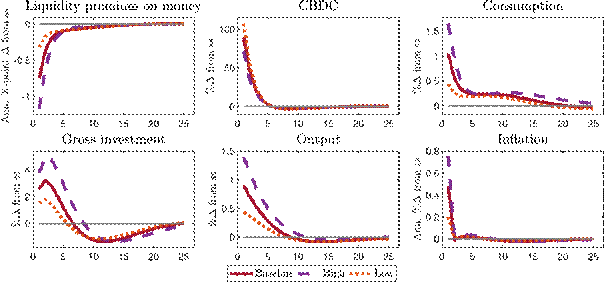
Figure 9: Responses to a 50 bps CBDC rule shock with CBDC for high and low CBDC rule parameter ?_m

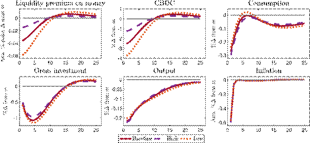
Figure 10: Responses to a contractionary 50 bps conventional monetary policy shock with CBDC for high and low CBDC rule parameter ?_m

Business cycle shocks

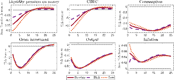
Figure 11: Responses to a 1% TFP shock with CBDC afor high and low CBDC rule parameter ?m

Financial shocks

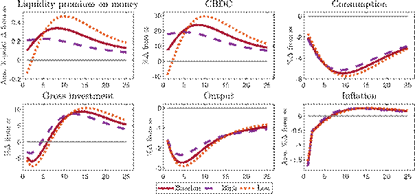
Figure 12: Responses to a 5% capital quality shock with CBDC for high and low CBDC rule parameter ?_m

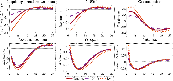
Figure 13: Responses to a negative 1% bank net worth shock with CBDC for high and low

CBDC rule parameter ?_m

Liquidity premium shocks

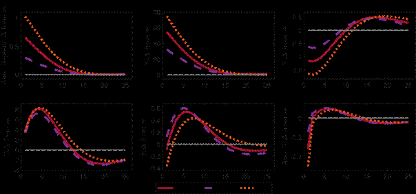
Figure 14: Responses to a 5% reduction in payment efficacy of deposits with CBDC for high and low CBDC rule parameter ?_m

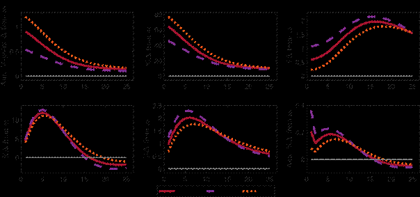
Figure 15: Responses to a 5% preference shock for DM consumption with CBDC for high and low CBDC rule parameter ?_m

A.2 Comparison to a money in the utility function approach

This section highlights the additional insights obtained from an explicit formulation of the medium of exchange function by comparing the results against a money in the utility function approach as pioneered by Sidrauski (1967). In New Keynesian models, the medium of exchange function is if at all mainly embedded via money in the utility (MIU) function setup, cashin-advance constraints or shopping time models. In contrast, we follow the New Monetarist paradigm (e.g. see Williamson and Wright, 2010) and spell out the medium of exchange function explicitly because it is central to central banks’ motivation to issue retail CBDC as a means of payment. This comes at the cost of some complexity. We assess the advantage of this approach by contrasting it against a MIU specification, which gives rise to similar household optimality conditions. For this, we shut down the decentralized market and replace it by an additively separable MIU specification, similar to Gross and Schiller (2021), but keep the framework and calibration otherwise the same.

The household problem with a MIU specification and without the decentralised market becomes

(37) s.t. C_t^CM + M_t + D_t + B_t = w_tL_t + T_t + R_t^MM_t-1 + R_t^DD_t-1 + R_t^BB_t-1 + ?_t where l and

?_l denote the elasticity and relative utility weight of real money balances respectively. The resulting optimality conditions for CBDC and deposits are similar to the optimality conditions derived in equations 27 and 28 for the case in which real money balances are constrained. This can be seen when the constrained CBDC optimality conditions are displayed side by side^[25]: (Constrained optimality condition NMNK)

compared to

(Optimality condition MIU)

Although the household optimality conditions look very similar, additional dynamics arise through the monetary search and matching environment and the resulting additional equilibrium conditions on DM consumption and prices. These are tightly linked to the available liquidity and thus also to the household optimality conditions. To quantitatively compare the differences in both frameworks, l is calibrated to be as close as possible to 1 and set to 0.999, while ?_l is set to 0.058 such that it creates the same liquidity premium and CBDC share in steady state as in the NMNK model.

Overall, this exercise shows that the additively-separable MIU specification misses important dynamics. In the MIU specification, the liquidity premium arises from exogenous specification of the liquidity convenience yield parameters in the utility function without more complex linkages. While the calibration ensures a comparable steady state baseline, the fluctuations in the liquidity premium in response to shocks are substantially lower. Less variation in the liquidity premium leads to very low fluctuations across CBDC and deposits, which is again consistent across shocks. The main insights are as follows:

Monetary policy shock: The response to a CBDC rule shock transmits substantially differently in the MIU specification. The change in the CBDC interest rate is almost fully transmitted to inflation and there is almost no response to the liquidity premium. It creates large fluctuations in money, consumption, investment and output and the increase in the CBDC share in the economy is almost twice as much. The large increase in investment can be attributed to the large increase in CBDC that is accommodated via capital security purchases. In response to a conventional monetary policy shock under the MIU specification, consumption fluctuates stronger, while investment fluctuates less. Overall, this leads to a similar output response on impact but which is subsequently somewhat more pronounced. The inflation response is substantially lower because of the strong DM inflation response in the NMNK model.

Business cycle shocks: In response to a capital quality shock, the liquidity premium and CBDC react very little. The fluctuations in consumption are greater, while the fluctuations in investment are less than in the NMNK model. Overall, it leads to similar output dynamics as in the NMNK, while deposit response and inflation dynamics are more similar to the case without CBDC.

Financial shocks: For financial shocks there are barely fluctuations in the liquidity premium and therefore little fluctuations in the level of CBDC. Deposits behave similarly to the NMNK model without CBDC. While output dynamics are more pronounced in the MIU specification, inflation dynamics are less pronounced which can be attributed to the missing DM which amplifies inflation dynamics. Impact on deposits and investment varies over the shock.

Liquidity premium shock: In the MIU specification the DM is absent and therefore we cannot simulate a shock to DM consumption preference, however we can simulate a shock to the usefulness of deposits providing liquidity. Yet, with the same shock calibration, barely any dynamics arise in the MIU specification.

Monetary policy shocks

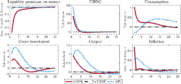
Figure 16: Responses to a 50 bps CBDC rule shock in NMNK with and without CBDC compared to a MIU specification with CBDC

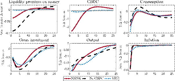
Figure 17: Responses to a contractionary 50 bps conventional monentary policy shock in NMNK with and without CBDC compared to a MIU specification with CBDC

Business cycle shocks

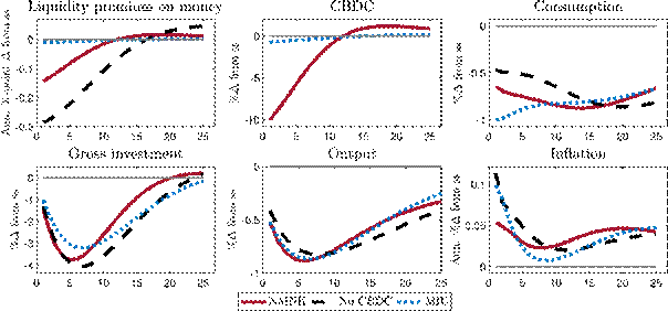
Figure 18: Responses to a 1% TFP shock in NMNK with and without CBDC compared to a MIU specification with CBDC

Financial shocks

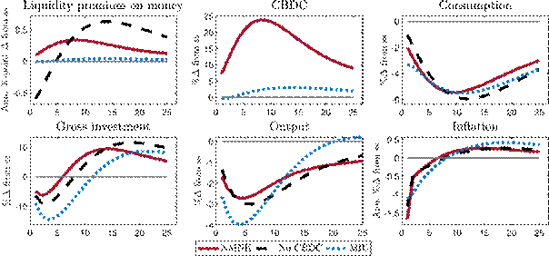
Figure 19: Responses to a 5% capital quality shock in NMNK with and without CBDC compared to a MIU specification with CBDC

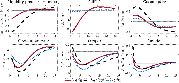
Figure 20: Responses to a negative 1% bank net worth shock in NMNK with and without CBDC compared to a MIU specification with CBDC

Liquiduty premium shocks

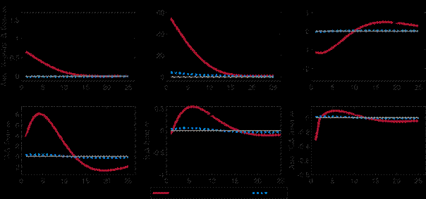
Figure 21: Responses to a 5% reduction in payment abitliy of deposits in NMNK with and without CBDC compared to a MIU specification with CBDC

A.3 Comparison to framework with neutral asset purchases

This stylized exercise aims to gain insight on the effects of the different channels by isolating the liability channel from the asset side channel through muting the CBDC asset side response. To construct a neutral” asset side response we assume that the central bank offsets CBDC issuance on the asset side by purchasing a government asset which cannot be held by any other agent in the economy. The government, as frictionless and passive entity in the economy, will pass any changes to the households via lump-sum taxation. In our model framework this channel is particularly muted as households have a linear disutility of labour in order to achieve equal asset holdings across agents after the DM. Although far from reality, such modelling enables us to mute the asset side implications of CBDC issuance. The calibration is set in a way to achieve the same steady state liquidity premium as in the baseline framework with CBDC. Due to the changes in the model framework, this produces a different steady state CBDC share in the economy.

Monetary policy shock: Overall, the response to monetary policy shocks under the neutral asset side scenario is in between the reactions with and without a CBDC in the baseline framework. While the increase in consumption to a CBDC rule shock is more pronounced, the response of investment is less pronounced an initially negative in the neutral asset side scenario.

Business Cycle Shocks: The response to a TFP shock is similar under a neutral asset side (NAS) and mostly in between the results of the baseline framework with and without a CBDC. As the central bank is not purchasing capital securities under a neutral asset side scenario, the reaction of deposits and investment is more similar to the model framework without a CBDC. In contrast, the inflation response of the NAS scenario is more similar to the baseline framework with CBDC.

Financial Shocks: In the baseline framework CBDC issuance is offset on the asset side through purchases of capital securities and thereby directly affects the response to a capital quality shock. As a result, in a neutral asset side scenario, the response to a capital quality shock is closer to the framework without CBDC. In contrast, the neutral asset side response to a net worth shock is more in between the case with and without a CBDC in the baseline framework, similar to the case under business cycles shocks.

Liquidity Premium Shock: Despite a similar stabilisation of the liquidity premium, CBDC issuance with a neutral asset side reduces fluctuations in response to liquidity premium shocks, for both a shock to deposit payment technology as well as a shock to the preference for DM consumption. The only exception to this is the DM preference shock reaction of inflation which is initially more pronounced under a neutral asset side.

Monetary policy shocks

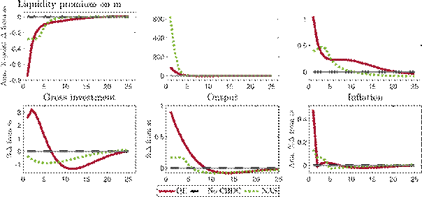
Figure 22: Responses to a 50 bps CBDC rule shock in NMNK with CBDC and a neutral central bank balance sheet asset side

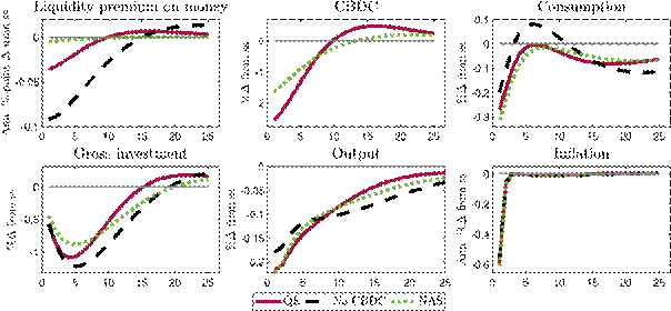
Figure 23: Responses to a contractionary 50 bps conventional monetary policy shock in NMNK with CBDC and and a neutral central bank balance sheet asset side

Business cycle shocks

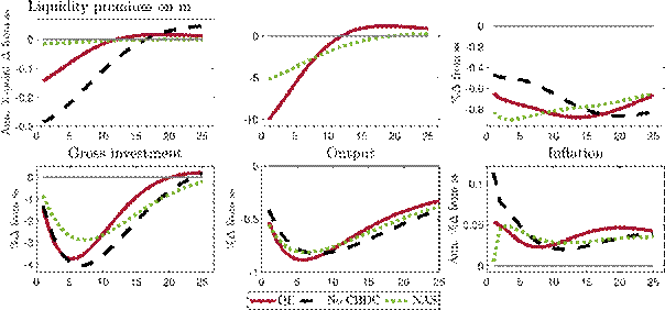
Figure 24: Responses to a 1% TFP shock in NMNK with CBDC and a neutral central bank

balance sheet asset side

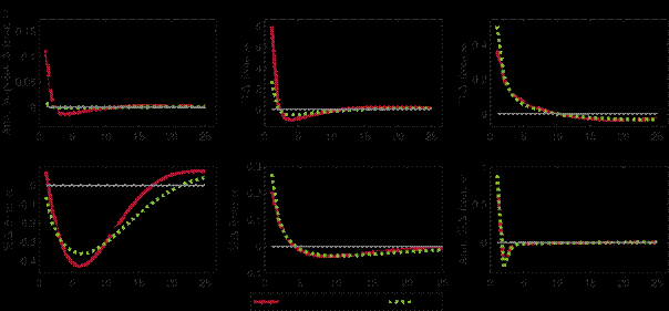
Figure 25: Responses to a 50 bps discount factor shock in NMNK with CBDC and a neutral central bank balance sheet asset side

Financial shocks

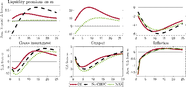
Figure 26: Responses to a 5% capital quality shock in NMNK with CBDC and a neutral central bank balance sheet asset side

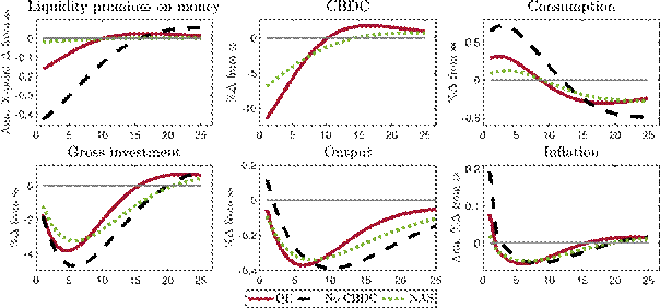
Figure 27: Responses to a negative 1% bank net worth shock in NMNK with CBDC and a neutral central bank balance sheet asset side

Liquidity premium shocks

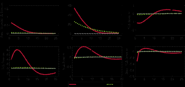
Figure 28: Responses to a 5% reduction in payment ability of deposits in NMNK with CBDC and a neutral central bank balance sheet asset side

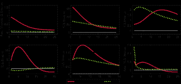
Figure 29: Responses to a 5% preference shock for DM consumption in NMNK with CBDC and a neutral central bank balance sheet asset side

B Detailed model calculation

B.1 Households

CM maximisation problem

The household’s value function in the CM is

s.t. the budget constraint

CtCM + Mt + Dt + Bt = wtLt + Tt + RtMM^t-1 + RtDD^t-1 + RtBBt-1 + ?t,

with

for buyers for buyers

M^{^}t = ?????? M_t + m^S_t for sellers and D^{^}t = ??^?D_t + d^S_t for sellers

M_t otherwise otherwise

where and are the amounts of CBDC and deposits spent in the DM and and are CBDC and deposits received in the DM. On aggregate, sellers get what buyers pay i.e.

mt = mBt = mSt and dt = dBt = dtS.

The problem yields the optimality conditions:

and envelope conditions

.

General DM maximisation problem

Besides the quantity and price of the DM good, to complete the optimality conditions we need to define the marginal value of the assets in the DM and . These can be determined by the marginal value of assets for the buyer and the seller:

VtDM = ?VtDM,B + ?VtDM,S + (1 - 2?)ßVtCM+1

? Vt,aDMt = ?Vt,aDM,Bt + ?Vt,aDM,St + (1 - 2?)Vt,aCMt for at = {Mt,Dt,Bt}

Buyer DM maximisation problem

The value function of the buyer

VtDM,B = DMmax {U(CtDM) + ßVtCM+1 (Mt - mt,Dt - dt,Bt,·)}

Ct ,mt,d_t

DM DM

s.t. P_t C_t = m_t + d_t,

0 ? m_t ? ?_MM_t,

0 ? d_t ? ?_DD_t

can be reformulated using the budget constraint m_t = P_t^DMC_t^DM -d_t and expressed as following Kuhn-Tucker optimization:

Lt = {U(CtDM) + ßVtCM+1 (Mt - PtDMCtDM + dt,Dt - dt,Bt)}

+ ?m,lt (PtDMCtDM - dt) + ?tm,h (?MMt - PtDMCtDM + dt)

+ ?d,lt (dt) + ?d,ht (?DDt - dt)

which yields the optimality conditions:

FOC CtDM :		= 0
FOC dt :		= 0

with

?m,lt (PtDMCtDM - dt) = 0, ?m,ht (?MMt - PtDMCtDM + dt) = 0, ?d,lt (dt) = 0,	?m,lt ? 0 ?m,ht ? 0 ?d,lt ? 0
?d,ht (?DDt - dt) = 0,	?d,ht ? 0

From the first-order conditions for C_t^DM, we can derive the demand function for goods in the DM, using from above:

From the first-order conditions for d_t we can derive the buyer’s optimality conditions for transactions with of CBDC and deposits, additionally using :

Moreover, we get that the marginal utility of money for a buyer in the DM is value of its transactions function plus the discounted continuation value of money balances:

Vt,MDM,Bt = ßVtCM+1,M^t + ?m,ht ?MMt

Vt,DDM,Bt = ßVtCM+1,D^t + ?d,ht ?DDt

Vt,BDM,Bt = ßVtCM+1,Bt

Seller DM maximisation problem

The sellers value function

VtDM,S(·) = maxDM {-C(CtDM) + ßVtCM+1 (Mt + mt,Dt + dt,Bt,·)}

C_t

? V_tDM,S(·) = maxDM {-C(C_tDM) + ßV_tCM₊₁ (M_t + P_tDMC_tDM - d_t,D_t + d_t,B_t,·)}

C_t

yields the optimality condition:

which implies that the price needs to equal the marginal cost of production relative to the marginal benefit of money in the CM. This can be interpreted as the supply function of the sellers.

Furthermore, we get that the marginal value of money for a seller in the DM is just the continuation value of the money balances he carries to the next CM:

Vt,MDM,St = ßVtCM+1,M^t

Vt,DDM,St = ßVtCM+1,D^t

Vt,BDM,St = ßVtCM+1,Bt

Equilibrium and terms of trade in the DM

Combining the demand function of the buyer with

the supply function of the seller yields

The equilibrium conditions in the DM can be divided into two regimes: an unconstrained and a constrained case. If there is enough liquidity in the DM, consumption is not constrained by money balances and one regime in which money balances limit DM consumption.

Unconstrained DM allocations

If money balances do not constrain DM consumption, the shadow price of additional liquidity is zero ?^m,l_t = ?^m,h_t = ?^d,l_t = ?^d,h_t = 0. In this case, equilibrium output equates marginal utility with marginal costs of the production

^UCtDM* ⁼ CCtDM*

Thus, unconstrained DM output does not depend on deposit and CBDC balances. In this case, there is no transaction value of an additional unit of money and the value of money in the DM just reflects the continuation value of it interest payments in the CM V_t,a^DM_t = ßV_t,a^CM_t for a =_t {M_t,D_t,B_t}. This implies that in this case, the interest rates on CBDC, deposits and bonds are equal. This leads, together with the DM output and DM prices, to the final CM and DM optimality conditions

Constrained DM allocations

Note that, as long as M_t > 0 and D_t > 0, it is not possible that both, lower and upper, constraint bind at the same time, i.e. ?^·_t^,h > 0 or ?^·_t^,l > 0. If the upper constraint is binding, the KuhnTucker multiplier of the lower constraint needs to be zero and vice versa. The DM production costs C(C_t^CM) are of convex nature and DM consumption utility U(C_t^DM) is of concave form. Given the DM equilibrium condition, this implies that if the buyer is constrained by its money holdings, it must be that C_t^DM < C_t^DM*. Therefore, if trade in the DM is constrained, it must be limited by the upper constraint, i.e. ?^m,h ? 0 and ?^m,l = 0, as long as the DM good has a positive valuation. However, equating the Kuhn-Tucker constraints of deposits and CBDC requires that if the upper constraints on CBDC is binding, the same needs to hold true for deposits i.e. ?^d,h ? 0 and ?^d,l = 0. This leaves us with following DM conditions that complete the DM market equilibrium

From this we can determine DM prices , DM consumption C_t^DM =

, and the shadow value of liquidity

and .

We can therefore now complete the household optimality conditions for CBDC,

deposits

and bonds .

B.2 Financial intermediaries

The banker’s objective is to maximise expected discounted net worth of the bank which evolves according to

with a balance sheet of the bank of

QtSj,tb = Nj,t + Dj. The maximisation problem is

where is the value of expand-

ing assets by one unit financed by deposits and is the value of expanding net worth by one unit holding assets constant.

The optimisation of the banker is subject to the moral hazard constraint . Under positive net worth, the constraint binds as long as 0 < µ^s < ?. A binding incentive constraint restricts the leverage ratio of the bank which can be expressed as

.

The evolution of net worth and assets can also be reformulated in terms of ?_t and as growth rates: .

Banking sector aggregates are obtained by the sum of the individual banks. Aggregate bank net worth comprises the net worth of banks in operation N_t^E and newly entering banks receiving an endowment :

.

C Overview of equilibrium equations

Description	Equation
CM consumption Stochastic discount factor DM consumption CBDC demand Deposit demand Bond demand	Households
	Banks
Balance sheet Leverage	QtStB = Nt + Dt

Continued on next page

Deposits

Dt = (?t - 1)Nt

Growth rate of net worth .

Growth rate of assets

Value of banks assets

Value of bank equity

Total net worth

Firms

CM production function

Capital securities

Return on capital

Depreciation function

Optimal capacity utilisation

Labour demand

Law of motion of capital

Net investment

Price of capital

Retail output

Final goods price dispersion

Inflation

Inflation optimal adjustment

Optimal price adjustment (1/2)

Optimal price adjustment (2/2)

Central Bank & Government Taylor rule

Continued on next page

Fisher equation bonds

Fisher equation CBDC

Fisher equation deposits

CB capital purchases

Mt = QtStCB

Government budget	G + RtBBt-1 + Tt = TtCB + Bt
Government bond issuance	G = Bt Aggregation
Total capital securities	St = StB + StCB

Central bank budget

CM GDP

DM GDP

DM prices

DM inflation

Total inflation

?t = (?tCM)1-s*(?tDM)s* Table 2: Overview of model equations in equilibrium

Total GDP

Acknowledgements

For helpful comments we thank Lukas Altermatt, Anna Andresen, Frank Heinemann, Manuel Munoz, Harald Uhlig, our discussants Martina Fraschini and Sebastian Zelzner as well as participants at seminars and conferences organised by the ECB, SNB and CIF, CEPR, CEBRA, EEA, TU Berlin, HU Berlin and Hong Kong Baptist University. We also thank Jonathan Schiller for sharing code with us.

This paper should not be reported as representing the views of the European Central Bank (ECB).

The views expressed are those of the authors which do not necessarily reflect those of the ECB and the authors are not part of the ECB’s digital euro project team.

Katrin Assenmacher

European Central Bank, Frankfurt am Main, Germany; email: katrin.assenmacher@ecb.europa.eu

Lea Bitter

European Central Bank, Frankfurt am Main, Germany; email: lea.bitter@ecb.europa.eu

Annukka Ristiniemi

European Central Bank, Frankfurt am Main, Germany; email: annukka.ristiniemi@ecb.europa.eu

---