Estimating the Euro Area output gap using multivariate information and addressing the COVID-19 pandemic

using multivariate information and addressing the COVID-19 pandemic

Disclaimer: This paper should not be reported as representing the views of the European Central Bank (ECB). The views expressed are those of the authors and do not necessarily reflect those of the ECB.

Abstract

We estimate the euro area output gap by applying the Beveridge-Nelson decomposition based on a large Bayesian vector autoregression. Our approach incorporates multivariate information through the inclusion of a wide range of variables in the analysis and addresses data issues associated with the COVID-19 pandemic. The estimated output gap lines up well with the CEPR chronology of the business cycle for the euro area and we find that hours worked, more than the unemployment rate, provides the key source of information about labor utilization in the economy, especially in pinning down the depth of the output gap during the COVID-19 recession when the unemployment rate rose only moderately. Our findings suggest that labor market adjustments to the business cycle in the euro area occur more through the intensive, rather than extensive, margin.

Keywords: Beveridge-Nelson decomposition, output gap, Bayesian estimation, multivariate information.

JEL classification: C18, E17, E32.

Non-technical summary

We estimate the euro area output gap by considering a relatively large set of fifteen variables, as well as addressing the unusual behavior of data associated with the COVID-19 pandemic. Our approach contrasts with most established methods of producing the output gap, such as the HP filter or a production function approach, which rely only on real GDP or at most a much smaller set of variables. By utilizing a larger information set, we are able to explicitly link the fluctuations in the output gap to a range of specific variables and particular economic shocks of

interest.

Our approach produces an estimated output gap that lines up well with the CEPR chronology of the business cycle for the euro area. Our estimated output gap is also comparable to other institutional estimates like that of the European Commission, but with far fewer restrictions imposed in estimation. We also find reasonable estimates throughout the COVID-19 pandemic. Because our empirical model allows us to decompose the output gap estimate into relevant sources of information, we are able to detect that hours worked is a particularly informative variable in terms of the output gap for the euro area and is crucially important in pinning down its depth during the COVID-19 recession. The result in terms of hours worked is unlike what has been found in the U.S.-centric literature, which typically shows the unemployment rate to be the most important measure of labor utilization when estimating the output gap. A possible reason for the difference is that labor market adjustments in the euro area occur more through the intensive, rather than extensive, margin, with the case in point being the much more moderate rise in the unemployment rate for the euro area than in the United States during the COVID-19

recession.

We also conduct a pseudo-real time analysis and find that our approach to estimating the output gap is comparatively reliable. With the caveat that our evaluation sample is short, and so should be viewed with some caution, our approach performs well relative to the HP filter. When comparing the pseudo real-time and final estimate, our approach leads to smaller revisions, a larger correlation between real-time and revised estimates, and a greater occurrence of the same sign for the estimates.

1      Introduction

The output gap, broadly defined as the deviation of real GDP from its trend, or potential output, is a crucial input into the formulation of monetary policy. It measures the degree of economic slack within the aggregate economy. While being a critical input for policy, the output gap is unobserved, and so has to be estimated.

In this paper, we estimate the output gap for the euro area. Our key contributions in doing so are to utilize information from a relatively large fifteen-variable set and addressing the occurrence of outlier observations associated with the COVID-19 pandemic. The latter issue should not be understated as real GDP growth in most of the world fell by over 20% quarter-on-quarter in annualized terms in 2020Q2 and then bounced back by similar magnitudes in the opposite direction in 2020Q3. To estimate the output gap, we apply the Beveridge and Nelson (1981)

(BN) decomposition based on a large Bayesian vector autoregression (BVAR), as proposed in Morley and Wong (2020), but making three modifications for the application to the euro area data with COVID outliers. First, we account for the fact that the euro area is an open economy and show that making the appropriate treatment of information in the foreign sector matters for estimating the output gap for the euro area, as opposed to simply following the typical closedeconomy assumption for the United States. Secondly, we address the effects of the COVID-19 pandemic by following Lenza and Primiceri (2022) to account for the outlier observations during the pandemic. The approach in Lenza and Primiceri (2022) makes sense for our setting given that we work with a BVAR. However, we make some modifications in our application due to using quarterly data, as opposed to the monthly data considered in Lenza and Primiceri (2022). Third, relative to Morley and Wong (2020), we work with a much shorter sample period as the euro area was only established in 1999Q1 and we consider the inclusion of data associated with the COVID-19 pandemic in our sample. The short sample makes the loss function based on out-of-sample forecasts that Morley and Wong (2020) adopt for calibrating the degree of shrinkage for the BVAR less suitable in the euro area setting. Instead, we adopt an alternative loss function to capture the idea that the shocks to the trend should not be excessively large, thus embedding the intuition of policy practitioners that the trend is smooth”. The new loss function appears to work well within our setting, where, in particular, the procedure is able to recognize that the COVID-19 pandemic in 2020Q2 and 2020Q3 was a large transitory drop in real GDP rather than a downward shift in trend.

Our approach produces an estimated output gap that lines up well with the CEPR chronology of the business cycle for the euro area. While our estimates are comparable with other institutional estimates, such as by the IMF or OECD, we also document key differences, including estimating a shallower output gap post-Global Financial Crisis to around 2016, implying potential output during that period, when the level of real GDP remained relatively flat, was not growing. In addition, we also find that hours worked is the key variable in terms of information about the euro area output gap. Notably, hours worked is extremely important in pinning down the depth of the output gap during the COVID-19 recession. The result in terms of the importance of hours worked stands in sharp contrast with the U.S. literature where various studies have shown that the unemployment rate is the main source of information for estimating the output gap (see, e.g., Morley and Wong, 2020; Berger, Morley and Wong, 2020; Fleischman and Roberts, 2012; Barbarino et al., 2020). A likely reason for the different result is that euro area economies adjust more through the intensive, rather than extensive, margin, perhaps due to labor market frictions. A key case in point is that the rise in the unemployment rate for the euro area during the COVID-19 recession was relatively modest when compared to changes in other economic indicators or to the rise the U.S. unemployment rate at the time.^[1]

The broader literature is replete with methods on how to estimate the output gap (e.g., see Canova, 2020, and the references herein). Methods that rely on applying filters to real GDP, such as the HP filter or Bandpass filter, require neither parameter estimation nor explicit accounting for information other than real GDP. These methods can therefore never incorporate a direct role where multivariate information, such as from the unemployment rate or hours worked, helps pin down the quantitative level of output gap. Within the broader literature, research estimating the output gap for the euro area is also somewhat scant relative to that for the United States. This is perhaps not entirely surprising given a history of only slightly over 20 years, with such a short sample presenting obvious econometric challenges. The extant econometric research of estimating output gaps for the euro area or euro area economies using multivariate information has largely employed unobserved components models with a small set of variables.^[2] Seen from the perspective of extremely short samples, it is perhaps even less surprising that previous studies do not consider large multivariate models and that our challenge of estimating a BVAR aiming to utilize information from fifteen variables to construct the euro area output gap should not be understated. Moreover, we also highlight that the outlier observations observed with the COVID-19 pandemic do not yet seem to have been satisfactorily addressed within the unobserved components framework and so our approach to dealing with these outliers should be of broader interest in its own right.^[3] Finally, we note that, given the Beveridge and Nelson (1981) decomposition is equivalent to an unrestricted unobserved components model (see Morley, Nelson and Zivot, 2003), the contrast to the extant research using unobserved components models is perhaps not as stark as it may at first appear.

The remainder of this paper proceeds as follows: Section 2 presents the multivariate BeveridgeNelson decomposition approach and details on the modeling features that deviate from Morley and Wong (2020), as well as describing the data used in our analysis. Section 3 discusses the main estimation results, the informational content of the various variables, including the important roles of hours worked and the foreign sector, and lastly a number of robustness checks.

Finally, Section 4 concludes with the key insights from our empirical analysis.

2        Methods and data

Our modeling framework builds on Morley and Wong (2020), who apply the BN decomposition based on a large BVAR to estimate the U.S. output gap. We first briefly present the approach proposed by Morley and Wong (2020), before motivating the modeling choices we make that deviate from them to address issues with the data for the euro area. We then describe the data.

Beveridge and Nelson (1981) define the trend of a time series, y_t, as the long-horizon conditional forecast minus any deterministic drift. The BN trend, ?_t^BN, where the long-run conditional expectation of the cyclical component goes to zero, is:

?_t^BN = lim Et[y_t+j - j · Et[?y_t]],    (1) j›?

where Et[?y_t] = µ is the deterministic drift or unconditional mean of the growth rate of y_t. In our application y_t is the natural logarithm of the euro area real GDP and ?y_t is its first difference, which approximates the quarter-on-quarter real GDP growth rate. Consider a VAR(p) forecasting model in the companion form:

                                                                                      X_t = FX_t-₁ + He_t,                                                                                 (2)

where X and x~_t represents a N × 1 vector of demeaned variables where x~_t ? x_t -µ and µ is an N ×1 vector of means for x_t.^[4] F is a companion matrix, e_t is a N ×1 vector of forecast errors, and H is a matrix that maps the forecast errors to the companion form. Let ?~y_t, or demeaned output growth, be the k^th element of x~_t. Defining s_k as a 1×Np selector vector with 1 as its k^th element and zero otherwise, Morley (2002) shows that the output gap, or the BN cycle of y_t can be calculated as as follows:

                                                                        .                                                                    (3)

At a high level, the methodology relies on specifying a BVAR, casting it into the form implied by Equation (2), and then subsequently applying Equation (3) to construct the output gap. Specifying a standard BVAR for a demeaned vector of variables:

x~_t = ?₁x~_t-₁ + ... + ?_px~_t-_p + e_t                     (4)  ,           (5)

where E(e^'_te_t) = ? and E(e^'_te_t-i) = 0 ?i > 0. The sample mean is used to demean the variables, which is basically equivalent to setting a flat prior on the unconditional means. Shrinkage is applied to the VAR coefficients using a Minnesota-type prior specification. Defining ?^jk_i as the slope coefficient of the i^th lag of variable k in the j^th equation of the VAR in equation (5), where the prior means and variances of the slope coefficients as follows:

(6)

(7) ,                otherwise,

with the variances ?_j² and ?_k² set to the variances of residuals from AR(4) models estimated using least squares for the corresponding variables as per the usual practice (e.g., Banbura, Giannone and Reichlin, 2010; Koop, 2013). Following the standard Minnesota prior structure, the factor  shrinks coefficients at longer lags.

? is a key hyperparameter and governs the degree of shrinkage with ? › 0 shrinking to the assumption that the variables in the VAR are independent white noise processes or, equivalently for all of the differenced variables in the VAR, independent random walk processes in their levels. Morley and Wong (2020) choose ? by minimizing the one-step ahead out-of-sample forecast error for real GDP growth. The issue is that parameter proliferation in the BVAR is a key source of potential overfitting, with overfitting leading to spurious forecastability. As Evans and Reichlin (1994) demonstrate that the forecastability of real GDP growth is the key ingredient in obtaining a particular estimated output gap, setting the shrinkage hyperparameter, ?, to minimize the overfitting of real GDP is a well-motivated approach.

Banbura, Giannone and Reichlin (2010) show how one can set a natural-conjugate prior with the prior implied by Equations (6) and (7). The natural conjugate-prior is convenient in our setting as, conditional on ?, all the posterior moments of the model can be calculated analytically without requiring MCMC methods to approximate the posterior distribution. This is an important efficiency gain as it enables one to choose ? in an out-of-sample forecast setting, re-estimating the model multiple times without needing to resort to MCMC methods. We note that Giannone, Lenza and Primiceri (2015) introduce an approach that estimates, rather than fixes, ?. However, the Giannone, Lenza and Primiceri (2015) approach involves evaluating the marginal likelihood of the whole BVAR system. As discussed in Morley and Wong (2020), because the interested is in the output gap, which is linked to the fit of the output growth forecasts, and not the whole BVAR system per se, using the Giannone, Lenza and Primiceri (2015) approach of estimating ? places too much weight on fitting the whole system rather than the object of interest (i.e., the target variable of log real GDP for estimating the output gap).

Results for a system-wide approach could also be quite sensitive to which variables are included in the system.

2.1       Modifications from previous modeling approach

We now discuss how our modeling approach deviates relative to Morley and Wong (2020) on three key dimensions.

2.1.1         Allowing for a foreign sector

Because the euro area is a relatively open economy, we include a foreign sector in the BVAR to allow for foreign shocks, similar to some of the existing open-economy literature (see, e.g., Zha, 1999; Justiniano and Preston, 2010; Kamber and Wong, 2020). Our approach is to use a twoblock foreign and domestic structure, where we treat the foreign block as being block-exogenous to the euro area. To set up a two-block structure, we first partition the vector x~_t in Equation

(4) to x~ where z^*_t and z_t are now N^* × 1 and [N - N^*] × 1 vectors of demeaned

foreign and domestic variables respectively. Throughout, we take the euro area as the domestic economy and thus rewrite the VAR in Equation (4) as:

? ? ? ? zt

=

21 p

? + ? ? ? A21

A22

?? ?, ?? ? ?t

(8)

? ? ? ?? ? z_t* ?11₁ 0 zt*-1

where the coefficients on the lags of z_t are now constrained to 0 in the equations for the variables in z_t^*. While the euro area is not really a small economy per se, we take the perspective that it is only small relative to the rest of the world given the size of the global economy is about five times larger than the euro area. We also view our restrictions as a pragmatic solution to allow us to identify foreign shocks by treating the foreign block as block-exogenous, thus allowing us to quantify the importance of foreign shocks in driving the euro area output gap.

On a more technical note, the zero restrictions mean that we lose the natural-conjugacy of the Normal-Inverse Wishart prior that Banbura, Giannone and Reichlin (2010) introduced for large BVARs. The loss of the natural-conjugate prior is non-trivial in our context because it was the speed of estimation of the posterior moments that enabled Morley and Wong (2020) to easily evaluate the out-of-sample forecasts across a variety of ?’s when choosing the optimal degree of shrinkage. In other words, the block-exogenous structure considered here imposes a very large computational cost.^[5] We return to this point later, as one would naturally ask whether it is worth paying the large computational cost for the sake of imposing block-exogeneity.

2.1.2             Treatment of outlier observations around the COVID-19 pandemic

A more recent issue is how to treat observations associated with the COVID-19 pandemic. As is now well-known, observations during the pandemic period can induce non-trivial changes to the estimated parameters for a BVAR. We take a pragmatic approach in dealing with the COVID-19 data following the suggestions of Lenza and Primiceri (2022). We first rewrite Equation (4) as

                                                                     x~_t = ?₁x~_t-₁ + ... + ?_px~_t-_p + s_te_t.                                                                (9)

The approach of Lenza and Primiceri (2022) treats s_t as a parameter during COVID-19 pandemic, where the role of s_t essentially allows the whole covariance matrix to scale up by a factor of s²_t during the pandemic period. Once conditioning on s_t, we can specify the BVAR as follows:

                                                              x~_t/s_t = ?₁x~_t-₁/s_t + ... + ?_px~_t-_p/s_t + e_t.                                                       (10)

As it should be clear, if s_t = 1 ?t, the model collapses back into the standard BVAR in Equation

(4). Lenza and Primiceri (2022) essentially specify three parameters to model the effects of COVID-19: one for March 2020, one for April 2020, and one to govern decay back to normal after April 2020. Within the context of a 6-variable monthly BVAR of the U.S. economy, their approach works relatively well. In our case, it is more appropriate to adjust their approach to the quarterly data we use. We similarly set three COVID parameters; one each of 2020Q1, 2020Q2, and 2020Q3. That is, we set s_t = 1 except for those three observations, where we estimate a different s_t for each of these three quarters. We do not model a decay parameter because we find that the variation post 2020Q3 appears to be back to pre-pandemic levels.^[6] On the other hand, we require one parameter each for 2020Q1, 2020Q2, and 2020Q3 because the data were characterized by different magnitude changes in many variables all three quarters, with much larger drops in many series in 2020Q2 than in 2020Q1 and large rebounds in 2020Q3.

Lenza and Primiceri (2022) extend Giannone, Lenza and Primiceri (2015) by modeling s_t in a hierarchical structure together with ? and jointly estimate all these parameters, where four parameters are jointly estimated using a fully Bayesian approach through drawing these parameters jointly in a Metropolis-Hasting step. We adopt a more pragmatic approach because a fully Bayesian approach is considerably less computationally efficient. In particular, as our previous discussion has alluded to, we need to be able to quickly evaluate the model across different values of ?, so re-estimating the model for various values ? is highly computationally intensive.^[7] Instead, we adopt a two-step approach, which is a hybrid of Bayesian and maximum likelihood estimation (MLE) approaches discussed in Lenza and Primiceri (2022). Lenza and Primiceri (2022) show how to concentrate s_t out of the likelihood function and so allow for estimation of the COVID parameters using MLE. Following this, we take a two-step approach where we first estimate our COVID parameters using MLE and then we reweight the data with the MLE estimate of s_t as per Equation (10). Then, it is straightforward to estimate a standard BVAR with the reweighted data. While one might naturally question moving between a frequentist and Bayesian approach from the first to second step, we verify this matters very little in our application and show later that our baseline estimates of the output gap are essentially identical to taking a fully Bayesian approach to estimating s_t when fixing ? at its chosen value for our baseline estimation. In terms of computational efficiency, our two-step approach is about a factor of 40 times faster than taking a fully Bayesian approach.^[8]

2.1.3           Loss function for setting the shrinkage hyperparameter

Finally, in terms of modifications from Morley and Wong (2020), we discuss the loss function in setting the shrinkage hyperparameter in Equation (6), ?. Morley and Wong (2020) calibrated ? to minimize the one-step ahead out-of-sample forecast error of output growth, with a key intuition underpinning this approach being to mitigate the possibility of overfitting output growth with a large BVAR. While the approach in Morley and Wong (2020) has proven to be reasonably useful within the context of estimating the output gap for the United States (see, e.g. Berger, Morley and Wong, 2020; Berger, Richter and Wong, 2022), it poses two challenges within the context of our application. First, we have a much shorter sample relative to working with U.S. data, and, second, the occurrence of the COVID-19 pandemic in the sample requires addressing specific challenges with forecasting outlier observations. The sample we consider is short due to the relatively recent launch of the euro area, meaning we have only slightly more than 20 years of observations to fit a reasonably sized VAR on, or around 90 quarterly observations.^[9]Given a 15-variable BVAR with 4 lags, the available 90 or so quarterly observations does not allow for a sufficiently long out-of-sample sample period with which to calibrate ?. Moreover, given that observations related to the COVID-19 pandemic are reweighted by s_t, it is not clear how to implement an out-of-sample forecast, as the model is, strictly speaking, forecasting the reweighted observations. One way around the problem of the short sample would be just to fix the value of the hyperparameter ?, as one often encounters in the BVAR literature, such as setting ? = 0.2 (e.g., see Carriero, Clark and Marcellino, 2015). Our results will show that this approach proves viable for the pre-COVID sample, but is less suitable during the pandemic.

As an alternative, we adapt an approach proposed by Kamber, Morley and Wong (2022) to our multivariate setting by choosing ? to minimize the variance of the change in trend. Implicitly, this means that we choose ? by imposing a relatively smooth trend. Kamber, Morley and Wong (2022) apply this criterion with their univariate BN filter and find it is helpful in addressing the COVID-19 outliers. In our setting, as our empirical results will show, minimizing the variance of the change in trend also appears to be a suitable way to deal with the COVID-19 recession, where real GDP fell by a lot, but the strength of the immediate rebound would a priori suggest that the trend did not change by much. We will later present results that show that other approaches of setting ? imply a large change in trend with the large fall of GDP, which while arguably plausible ex ante, appears unlikely ex post given what we now know about the dynamics of real GDP growth post-2020Q2.

2.2     Data

We include fifteen stationarized variables in our BVAR for the period from 1999Q1 to 2021Q2. The raw variables in the foreign block are U.S. real GDP and the real price of oil, while the raw variables in the domestic block are euro area real GDP, industrial production, employment, housing permits, CPI, the policy rate, hours worked, the term spread, capacity utilization, the unemployment rate, PMI, the risk spread, and the real effective exchange rate. When appropriate, the data are transformed to be stationary. The appendix provides full details of the data sources in Table A1 and time series plots of the raw and stationarized data in Figures A1 and A2, respectively.

3      Results

3.1     Baseline results

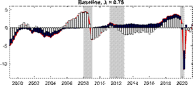
The top panel of Figure 1 presents the estimated output gap obtained for our 15-variable BVAR with ? = 0.75, which is chosen based on minimizing the variance of the estimated trend shocks over the whole sample. Overall, our estimated output gap for the euro area accords well with all turning points of the business cycle as dated by CEPR ever since the monetary union came into existence. Our estimated output gap experiences a large drop during the COVID-19 recession, with an estimated output gap of -10% in 2020Q2. Notably, the large drop is not persistent, as the output gap experiences a large bounce-back in 2020Q3, in line with the reversal of the large decrease in real GDP in 2020Q2 that can be related to the lockdowns to mitigate the initial spread of the virus and the subsequent opening up of the restricted sectors of the economy. Our output gap also lines up with the other two recessions in the sample in 2008/09, associated with the Global Financial Crisis (GFC), and 2011/2013, associated with the European sovereign debt

crisis.

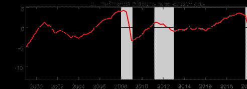
The bottom panel of Figure 1 compares our estimated output gap with external institutional estimates. We note that the institutional estimates by the OECD, European Commission (EC), and the IMF are based on annual data, and so might not be fully comparable to our estimate. All three institutions base their estimates off a framework that assumes a production function for the total economy and defines the output gap as the difference between actual output and the estimated trend according to the production function. UCM refers to estimates for an unobserved Figure 1: Baseline results Estimated output gap for the euro area

b. Comparison against external estimates of the output gap

Notes: The shaded bars represent CEPR dating of recessions. The output gap is measured as a percentage deviation from trend or potential GDP. BN refers to our baseline estimate using Beveridge-Nelson decomposition; HP filter refers to Hodrick-Prescott filter; UCM refers to an unobserved components model by T´oth (2021).

components model by ECB staff based on quarterly data. We also compare our results against an output gap constructed using the HP filter with a typical smoothing parameter of 1600 for quarterly data. Our estimated output gap aligns reasonably closely with the external estimates, as well as the HP filter estimate. That said, a key departure is that the institutional estimates consistently estimate a much lower output gap since the end of the Great Recession relative to our estimate, and also to the HP filter. In particular, the institutional estimates of the output gap at the trough of the euro area crisis are roughly similar to the depth of the output gap during the Great Recession, whereas ours has largely recovered. We note that real GDP in the euro area from the trough of the Great Recession to the trough of the European debt crisis only grew by 2.5%, which is roughly 0.66% per annum. From our estimates of the output gap, this implies that the external institutions’ estimated trend growth is 4-5% (approx. 1.3-1.6% annually) at a time when real GDP largely stagnated. In other words, our estimate implies flat potential output growth during the Great Recession, whereas the institutional estimates largely assume trend growth to be growing at a fast rate, even though actual output stagnated for 8-9 years. This is also another reason why the HP filter, like our approach, estimates a much smaller gap during the European debt crisis and thereafter. Because real output growth stagnated, implied potential growth for the HP filter also stagnated. We note that related work by Hasenzagl et al. (2019) suggests there was little slack in the euro area by 2017 and they estimate the output gap to have largely closed by 2017, possibly peaking in 2020Q1. While the timing of our increase in the output gap pre-dates theirs by about a year, our findings suggest a similar interpretation that the institutional measures may have been overly optimistic in terms of their estimates of potential output after the Great Recession.

3.2         Effects of COVID adjustments and shrinkage hyperparameter

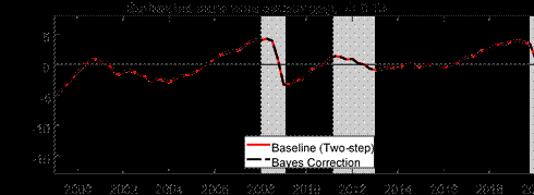
Because most of our modifications from Morley and Wong (2020) are aimed at dealing with data associated with the COVID-19 pandemic, we next turn our attention to how these modifications affect the estimated output gap during the COVID-19 recession, as well as considering the robustness of estimates beforehand. The top panel of Figure 2 illustrates the importance of the choice of modeling strategies for dealing with the high volatility of the data around the onset of the pandemic. Our baseline is the two-step approach of estimating different variances in the key quarters of 2020 and standardizing the data based on these estimates before estimating the

BVAR. The blue dotted line presents estimates that do not account for changes in volatility (i.e., it fits the whole BVAR without considering s_t in Equation (10) or, equivalently, setting s_t = 1 even during the COVID-19 recession). We keep the shrinkage hyperparameter constant to focus on how allowing for a change in volatility deals with the COVID data. Without an explicit treatment for the outlier observations associated with the COVID-19 pandemic, we see a larger pre-COVID output gap, indicating that the inclusion of data from during the COVID-19 pandemic without any adjustment would lead to non-trivial changes in the estimated model dynamics through changes in the BVAR parameters, an observation which mirrors the description of what Lenza and Primiceri (2022) observe with their 6-variable BVAR for the United States. We also explore an alternative strategy suggested by Lenza and Primiceri (2022), where one may consider estimating the model parameters with just the pre-COVID data to retain the pre-COVID dynamics for forecasting and impulse response analysis (see the black line). We find this strategy may be a reasonable compromise in our setting if one does not want to consider modeling the COVID data. There are some marginal differences around the pandemic, where estimating parameters with data up until 2019Q4 leads to a slightly lower gap before the pandemic, while the gap in 2020Q2 is a bit shallower than with our two-step approach. We nonetheless note that the approach of estimating parameters only up to 2019Q4 will become increasingly indefensible over time the further we get from 2020Q2. We, therefore, see our twostep approach as being more enduring going forward, especially as samples extend beyond the COVID-19 pandemic. Moreover, we note that our sample is quite short relative to the application by Lenza and Primiceri (2022), so an explicit treatment of the outlier observations during the

COVID-19 recession should be preferable to simply estimating parameters until 2019Q4 only.

Figure 2: Effects of COVID adjustments

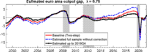
Notes: The shaded bars represent CEPR dating of recessions. The output gap is measured as a percentage deviation from trend or potential GDP.

A reasonable question is what would happen if we did not adopt the two-step approach, but rather did a full Bayesian estimation of the COVID parameters, as done in Lenza and Primiceri (2022). In particular, our two-step approach is an approximation since our estimation conditions on the COVID parameters, which are random variables, rather than treating them as random variables, as one would in a fully Bayesian treatment. The bottom panel of Figure 2 presents a comparison of results for our two-step approach and fully Bayesian estimation given a fixed ? = 0.75. Essentially, the two are indistinguishable. A key intuition of why this happens is because, with the pandemic, the increase in s_t is so large during the COVID-19 recession that the COVID observations are effectively reweighted to extremely small values even though the estimation methods yield different estimates for s_t.^[10] Because we scale by very large numbers whether we do the two-step or a fully Bayesian treatment, either strategy ends up with very similar estimated output gaps. We note, though, that the two-step approach, while an approximation, is computationally about 30 times more efficient than a fully Bayesian treatment of the COVID parameters. As both approaches turn out to produce results that are virtually indistinguishable, we thus view the efficiency gain as a good reason for us to adopt the two-step approach when needing repeated calculations, such as when determining the optimal ? to minimize the variance of the change in trend.

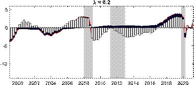
Next, we explore the effects of changing the shrinkage hyperparameter on the estimated output gap during the COVID pandemic, as well as beforehand. The top panel of Figure 3 presents our baseline results with ? = 0.75 against those for some other choices of the hyperparameter. The other choices for ? are 0.08 correponding to the value for U.S. real GDP in Morley and Wong (2020), 0.2 corresponding to the value suggested in Carriero, Clark and Marcellino (2015), and 0.9 to determine what happens as shrinkage is relaxed further towards MLE. Consistent with the Minnesota-type prior structure, more shrinkage (i.e., smaller ?) reduces the amplitude of the output gap, as the prior shrinks towards real GDP being modeled as a random walk with no cyclical component. Relaxing the shrinkage more to ? = 0.9 has barely any impact on the estimated output gap compared to our baseline case, suggesting our baseline shrinkage of ? = 0.75 is already fairly loose. The most notable effect of ? on the estimates is in terms of the COVID recession, where the smaller values of 0.08 and 0.2 produce only a small negative estimated output gap. The bottom panel of Figure 3 reveals that a small negative output gap during the COVID-19 recession translates into a large drop in the estimated trend for ? = 0.2, Figure 3: Effects of changing the shrinkage hyperparameter

Notes: The shaded bars represent CEPR dating of recessions. The output gap is measured as a percentage deviation from trend or potential GDP. Real GDP is reported in levels and normalized to 100 in 1999Q1.

while our baseline case of ? = 0.75 based on smoothing the trend has the much more intuitive result that the large fall in real GDP was largely transitory rather than a downward shift in

trend.

3.3      Informational content of variables

A particular feature of our modeling approach is that the multivariate nature of the model conveniently offers an economic interpretation through the decomposition of the output gap into sources of forecast errors or identified structural shocks. From Equation (3) and defining ?_i = Fⁱ(I-F)^-1, recursive substitution yields (see Morley and Wong, 2020):

t-1

                                                                    cBNt                = -sknX?i+1Het-i)o.                                                                     (11)

i=0

Equation (11) provides some intuition that the estimated output gap via the multivariate BN decomposition is simply a linear function of the historical forecast errors contained in e_t-i.

Consequently, we can back out the contribution of each variable’s forecast error to the BN cycle. Figure 4 presents the standard deviations of the informational contributions from each of the fifteen variables in the baseline model.^[11] We observe that almost every variable contributes non-negligibly to the estimated output gap, perhaps excepting the term spread and the PMI. We highlight two key insights from the informational decomposition. First, of the domestic variables, hours worked comes out as the most important in providing information about the estimated output gap, even in the presence of other labor market variables in the model such as the unemployment rate and employment. This result stands in sharp contrast to the analysis of Morley and Wong (2020), who show that the unemployment rate provides almost all of the useful information needed to estimate the U.S. output gap, a result that is also reflected in Berger, Morley and Wong (2020), and even in other modeling approaches used for estimating the U.S. output gap, such as Barbarino et al. (2020) and Fleischman and Roberts (2012). Second, the foreign block of variables, even though there are only two variables, accounts for a reasonably large share of information used to estimate the euro area output gap, highlighting the relevance of our approach considering the open-economy setting.

3.4      The role of hours worked

While the standard deviations used for the informational decomposition in Figure 4 provide useful clues as to which variables have been important on average, they may mask periods where certain variables have particularly sizeable contributions to the estimated gap. We thus also look at an historical informational decomposition, where we are effectively plotting the time series of the components described by Equation (11). To maintain readability, the top panel of Figure 5 presents the share of the forecast errors of hours worked (and the other 14 variables grouped together). Notably, hours worked is an important variable for providing information about the depth of the output gap during the COVID-19 recession. We see that a large component of the negative output gap during the COVID recession can be attributed to information about hours worked. Recall that this is in addition to other labour market variables such as unemployment and employment being in the model. We also note that hours worked no longer contributes much Figure 4: Informational content of variables

Notes: Units are standard deviations. Contributions to the estimated output gap for each variable are calculated taking the standard deviation for the role of each forecast error from Equation (11).

in 2020Q3, which suggests the bounce-back of hours worked has also provided information about output going back to trend. In the bottom panel of Figure 5, we consider the same historical informational decomposition, but now with ? = 0.2. For most of the sample, we can see that the share of hours worked mirrors that for our baseline model with ? = 0.75, re-emphasizing that, within a wide range, the specific value of the shrinkage hyperparameter has a meaningful impact on estimates only during the COVID-19 recession. Notably, the difference in the role of hours worked is by far most stark in the pandemic. Hours worked, while still important in the model with ? = 0.2, has a smaller negative contribution than in the baseline case, which results in the model with ? = 0.2 estimating a much smaller negative output gap in 2020Q2. Therefore, another way of understanding our results in terms of why we need to shrink less than typically done in other studies in order to produce an intuitive estimated output gap during the COVID-19 recession is that the shrinkage hyperparameter is allowing” a greater degree of forecastability from hours worked to real GDP growth, which is important in pinning down the Figure 5: The role of hours worked

	Other Variables Hours
	Other Variables Hours

Notes: The shaded bars represent CEPR dating of recessions. The output gap is measured as a percentage deviation from trend or potential GDP. The decomposition of the role of hours worked and the other variables is calculated using Equation (11).

quantitative effects of the COVID-19 recession on the output gap.

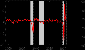
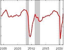
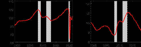
The time series plots for some select variables from the model are presented in Figure 6. These provide further context for why hours worked mattered so much in pinning down the depth of the output gap during the COVID-19 recession. The top left subplot shows that relative to the unemployment rate, which is important in pinning down the depth of the output gap in the United States, the unemployment rate rose very little in the euro area during the COVID-19 recession, suggesting much of the labor utilization adjustment in response to the pandemic occurred on the intensive, rather than extensive, margin. Certainly, hours worked were not the only variable that experienced a large drop. Indeed, industrial production growth and capacity utilization, two variables that are also in our model, fell by a lot during the Figure 6: Time series plots for select variables

Industrial Production Growth

Capacity Utilization

                                               Hours Worked                                                          Unemployment Rate

Notes: The shaded bars represent CEPR dating of recessions. Hours worked and capacity utilization are expressed in index terms. Industrial production growth is reported in percentage terms.

COVID-19 pandemic. However, the magnitude of these falls was comparable to levels that they fell during the Global Financial Crisis recession in 2008/09. Because the fall in real GDP during the COVID-19 recession was larger by an order of magnitude relative to the Global Financial Crisis or also during the recession associated with the European debt crisis, it is clearly necessary to also consider a variable that displays similar such dynamics when pinning down the depth of the output gap during the COVID-19 recession, which visually inspecting the plots in Figure 6, provides some intuition for why hours worked is such a crucial variable in providing information about the level of the output gap.

3.5       The role of the foreign sector

Another feature of our modeling approach is that we allow for two blocks, foreign and domestic, in the BVAR, with the foreign block being treated as block-exogenous. We thus explore the importance of block-exogeneity for our results. Understanding the implications of block-exogeneity also has practical modeling implications. Because the block-exogeneity structure means we move away from the natural conjugate prior used by Morley and Wong (2020), the block-exogenous structure introduces a large degree of computational inefficiency because the model posterior distribution no longer has a closed-form solution and we need to resort to MCMC methods for estimation. Therefore, it is natural to explore the benefits in return for this large inefficiency cost. The top panel of Figure 7 compares our baseline model with a model which does not impose block-exogeneity. We can see that there are sizable differences in parts of the sample. In particular, not imposing block-exogeneity implies a larger pre-COVID gap and a more negative gap during the pandemic. Nonetheless, as our previous discussion has alluded to, one could argue that a looser shrinkage post-COVID may be unfair to evaluate a model which does not allow for block-exogeneity since one would not choose such a large shrinkage hyperparameter without the presence of COVID in the sample. Therefore, in the bottom panel of Figure 7, we compare the estimated gap with and without block-exogeneity but only using data up to 2019Q4, and a shrinkage hyperparameter one might have used prior to COVID, ? = 0.2. We still observe that not allowing for block-exogeneity results in a much larger pre-COVID output gap, suggesting that there are more general benefits from allowing for block-exogeneity in our modeling approach.

While we show in Figure 7 that imposing block-exogeniety leads to meaningful differences in the reduced form VAR parameters and thus alters the estimated output gap, our approach also embeds the flexibility to do structural analysis unlike some other trend-cycle decompositions (e.g., HP filtering). Block-exogeneity naturally leads to a structure where we can decompose the output gap in foreign and domestic shocks, as implied by Equation (8).

Figure 8 presents a decomposition of the baseline multivariate BN gap into foreign and domestic shocks. Overall, a substantial portion of the cyclical fluctuations for the euro area economic growth are driven by foreign shocks given its openness and against the background of an increased level of globalization over the sample period. During the COVID recession in 2020Q2 for example, one-third of the large negative drop in output gap is accounted for by foreign shocks, with the virus spreading also in the rest of the world, but two-thirds of the drop was due to domestic conditions, mostly attributable to the enforcement of lockdown measures. In the years before the COVID outbreak, the shock decomposition also indicates that the euro area output gap was bolstered by economic conditions abroad. Similarly, it also shows that the Figure 7: Effects of block-exogeneity

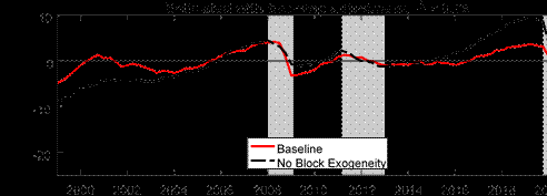
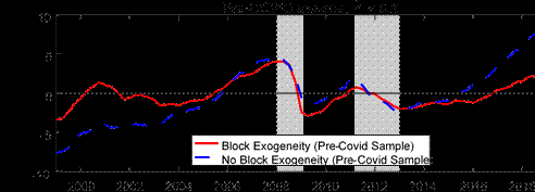
Notes: The shaded bars represent CEPR dating of recessions. The output gap is measured as a percentage deviation from trend or potential GDP.

negative output gap during the GFC recession was mainly driven by spillovers from outside the euro area, but the negative effects of the output gap during European sovereign debt recession were mostly driven by economic conditions within the euro area.

3.6     Reliability

Finally, we explore real-time reliability of our modeling approach. We compare with the HP filter given it is a widely-used approach to estimating the output gap. The top two panels of Figure 9 present vintages of pseudo real-time estimates of the output gap for our approach and for the HP filter. That is, with each new observation of quarterly real GDP, we re-estimated the model. We note that, for our procedure, ? is re-optimized for each pseudo real-time sample by minimizing the variance of trend shocks to get a sense of how the criteria would have behaved in real-time with pre-COVID data. The plots in the top two panels display the pseudo real-time Figure 8: Decomposition of the euro area output gap estimate into foreign vs. domestic shocks Shock Decomposition (Two-Step)

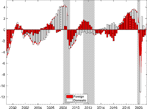
Notes: The shaded bars represent CEPR dating of recessions. The output gap is measured as a percentage deviation from trend or potential GDP.

output gap estimates from 2014Q1. A caveat to our analysis is that, because the sample is very short, we do not have a long evaluation sample to assess reliability, so these results should be interpreted as being suggestive at most.^[12] In general, the revisions to the output gap estimates are non-trivial. With such analysis, it is often a judgment call on what implies a final” estimate since these are estimated models, and so parameters can continue to change in the future. The usual practice is to take the final vintage as final” and omit the last five years for evaluation since the end of sample estimates are often those that change a lot. Therefore, while we present pseudo real-time estimates, it has been less than 3 years since the COVID-19 recession, and so one should not yet evaluate the revision properties during the COVID period and beyond.

Nonetheless, we uncover some interesting patterns in terms of revision properties. Focusing Figure 9: Pseudo real time estimates of the euro area output gap

                                          Multivariate BN Gap                                                               HP Filter

                      2014           2016           2018           2020                         2014           2016           2018           2020

Real Time Gap

Notes: The shaded bars represent CEPR dating of recessions. The output gap is measured as a percentage deviation from trend or potential GDP. The solid line in the upper two panels are the estimated output gaps per the respective method with data up to 2021Q2. The dotted line in the upper two panels represent the estimated pseudo real-time output gap per the respective methods using an expanding window of data.

on the period from 2014 to just before the pandemic, each subsequent vintage post-pandemic seems to revise the real-time gap upwards. For our approach, this is because we increasingly loosen the shrinkage hyperparameter over time. For the HP filter, the revisions are likely due to known end-point issues. During the COVID-19 recession, our measure does take about one quarter to learn about the precise depth of the output gap.^[13] More formally, we also assess reliability relative to the HP filter by drawing on Orphanides and Norden (2002) to consider the correlation and size of revisions between the real-time and ex-post estimated output gap, as well as whether the ex-post and real-time estimate have the same sign.

Table 1 reports the revision statistics of our gap relative to the HP filter. Taking a sample up until 2019Q4, our multivariate approach to estimating the output gap outperforms the HP filter whether in terms of correlation, size of the revisions (RMSE), or inferring the same sign. The 0.94 correlation between the real-time and ex-post measure of the gap even though we allow ? to change in pseudo real-time is a strong indication that the multivariate information is helpful in inferring the final output gap, even if the gap is somewhat revised. The pre-pandemic sample also suggests our method has smaller revisions relative to the HP filter, whereas our approach has an RMSE that is about 15% smaller. Notably, our method yields a sign of the output gap that is the same as the ex-post sign 83% of the time, while the HP filter infers the wrong sign more than half the time, possibly due to the known end-point issues. Taking the pandemic into account may suggest some improvement in the revision properties of the HP filter, although given that there are relatively few observations since the onset of the pandemic, these statistics may be revised further as we are at the very end of the sample and also noting that standard methods of evaluating revision properties often omit the last five years of the evaluation sample

(see Orphanides and Norden, 2002; Kamber, Morley and Wong, 2018).

Table 1: Revision statistics - 2014Q1-2019Q4

	Multivariate BN	HP filter
Correlation	0.94	-0.69
RMSE	1.59	1.85
Same sign	0.83	0.42

Notes: Correlation refers to the correlation between the pseudo real-time and ex-post estimate of the output gap. RMSE is the root mean square of the difference between the pseudo realtime and ex-post estimate of the output gap. Same sign is the proportion of times where the pseudo real-time and ex-post estimate of the output gap share the same sign.

Overall, our approach displays reasonable revision properties, at least when compared with the widely-used HP filter, although we again reiterate the caveat that the short evaluation period means we should only treat these results as suggestive at best. Ideally, one would need a longer sample to do real-time analysis, but the results from evaluating with a short sample so far appear supportive of our approach in comparison to the HP filter.

4      Conclusions

We apply the Beveridge-Nelson decomposition based on a large BVAR in order to obtain an estimated output gap for the euro area. Our modeling approach extends the framework proposed by Morley and Wong (2020) by addressing the COVID-19 pandemic and also considering the relatively short sample given the relatively recent launch of the euro area. Our approach is successful in estimating an output gap for the euro area that lines up well with the CEPR chronology of the business cycle and is similar to other institutional estimates, but does not rely only on real GDP data or a production function approach with only a few variables.

With the caveat that any real-time evaluation in our setting is hamstrung by the short sample, our approach is promising in that it demonstrates reliability properties that are better than the widely-used HP filter. More importantly, we show how to handle the unusual data dynamics associated with the COVID-19 pandemic, as well as including a foreign sector to account for the open economy feature of the euro area.

From our empirical analysis, we find that data on hours worked contains important information in pinning down the depth of the euro area output gap during the COVID-19 recession. This result stands in sharp contrast to the United States, for which the unemployment rate appears to be the most important source of information in pinning down the output gap (see

Morley and Wong, 2020; Fleischman and Roberts, 2012; Barbarino et al., 2020).

References

Banbura, Marta, Domenico Giannone, and Lucrezia Reichlin. 2010. Large Bayesian Vector Auto Regressions.” Journal of Applied Econometrics, 25(1): 7192.

Barbarino, Alessandro, Travis J Berge, Han Chen, and Andrea Stella. 2020. Which

Output Gap Estimates Are Stable in Real Time and Why?” Board of Governors of the Federal Reserve System.

Berger, Tino, and Christian Ochsner. 2022. Tracking the German Business Cycle.” Available at SSRN 4075961.

Berger, Tino, James Morley, and Benjamin Wong. 2020. Nowcasting the output gap.” Journal of Econometrics.

Berger, Tino, Julia Richter, and Benjamin Wong. 2022. A unified approach for jointly estimating the business and financial cycle, and the role of financial factors.” Journal of Economic Dynamics and Control, 136: 104315.

Beveridge, Stephen, and Charles R Nelson. 1981. A new approach to decomposition of economic time series into permanent and transitory components with particular attention to measurement of the ‘business cycle’.” Journal of Monetary economics, 7(2): 151174.

Bobeica, Elena, and Benny Hartwig. 2021. The COVID-19 shock and challenges for time series models.” European Central Bank Working Paper Series 2558.

Busetti, Fabio, and Michele Caivano. 2016. The trendcycle decomposition of output and the Phillips Curve: Bayesian estimates for Italy and the Euro Area.” Empirical Economics, 50(4): 15651587.

Camba-Mendez, Gonzalo, and Diego Rodriguez-Palenzuela. 2003. Assessment criteria for output gap estimates.” Economic modelling, 20(3): 529562.

Canova, Fabio. 2020. How do I extract the output gap?” Sveriges Riksbank Working Paper

Series.

Carriero, Andrea, Todd Clark, and Massimiliano Marcellino. 2021. Nowcasting Tail Risk to Economic Activity at a Weekly Frequency.” C.E.P.R. Discussion Papers CEPR Discussion Papers 16496.

Carriero, Andrea, Todd E. Clark, and Massimiliano Marcellino. 2015. Bayesian VARs: Specification Choices and Forecast Accuracy.” Journal of Applied Econometrics, 30(1): 4673.

Evans, George, and Lucrezia Reichlin. 1994. Information, forecasts, and measurement of the business cycle.” Journal of Monetary Economics, 33(2): 233254.

Fleischman, Charles A, and John M Roberts. 2012. From Many Series, One Cycle: Improved Estimates of the Business Cycle from a Multivariate Unobserved Components Model.”

Giannone, Domenico, Michele Lenza, and Giorgio E. Primiceri. 2015. Prior Selection for Vector